每次回家视力养护都有一个小妹妹,不到十岁,我很喜欢她,本来我以为是因为年纪到了,基因开始作祟喜欢小朋友,昨晚我突然想到了可能是因为我被小朋友的坦诚所吸引,比如,她妈妈说不喜欢宠物,因为她女儿喜欢,所以养了,小朋友听到后很难过过来告诉妈妈,妈妈,你说你喜欢小动物,妈妈你说你喜欢小动物,小朋友害怕因为自己喜欢但是妈妈不喜欢,所以很坦诚的表达了自己也喜欢妈妈喜欢,她以为她妈妈说了喜欢就真的喜欢了,她也就没有心理负担了,哈哈,越来越喜欢坦诚的人或者事,可能我也越来越坦诚面对自己和这个世界了
开源地址:https://github.com/JyAether/easytensor
项目概述
我认为不实现一遍都不算是真正理解本质, EasyTensor 是我最近一个基于 Python 的轻量级深度学习框架,旨在提供类似 PyTorch 的 API 设计,让深度学习变得更加简单易用。项目支持自动微分、多维数组运算、GPU 加速和智能内存管理,以及 Transformer,Bert 等主流模型也提供了完整的实现细节,同时由于深度学习计算图过于复杂,对于初学者,我提供了兼容层 V1 版本,基于原始Node实现,方便大家理解深度学习的计算逻辑。
核心特性
- 自动微分: 完整的反向传播机制
- GPU 加速: 基于 CuPy 的 CUDA 支持
- 内存管理: 智能内存池和自动垃圾回收
- 模块化设计: 高度可扩展的神经网络模块
- 向后兼容: 保留 v1 版本接口,确保平滑升级
项目架构
目录结构总览
EasyTensor/
├── core/                    # 核心模块
│   ├── tensor.py           # 核心 Tensor 类
│   ├── device.py           # 设备管理
│   ├── model_io.py         # 模型保存和加载
│   ├── nn/                 # 神经网络模块
│   ├── data/               # 数据处理
│   ├── optim/              # 优化器
│   ├── utils/              # 工具模块
│   └── v1/                 # 兼容层
├── test/                   # 测试和示例
├── biz/                    # 业务示例
└── utils/                  # 绘图工具


EasyTensor/
├── core/                    # 核心模块
│   ├── tensor.py           # 核心Tensor类
│   ├── device.py           # 设备管理
│   ├── model_io.py         # 模型保存和加载
│   ├── nn/                 # 神经网络模块
│   │   ├── tensor_nn.py    # 基础神经网络层
│   │   ├── modules/        # 具体模块实现
│   │   │   ├── conv.py     # 卷积层
│   │   │   ├── embedding.py # 嵌入层
│   │   │   ├── pooling.py  # 池化层
│   │   │   └── rnn.py      # 循环神经网络
│   │   ├── attention.py    # 注意力机制
│   │   ├── bert_gpt.py     # BERT/GPT模型
│   │   ├── transform.py    # Transformer模型
│   │   └── distill.py      # 知识蒸馏
│   ├── data/               # 数据处理
│   │   ├── dataloader.py   # 数据加载器
│   │   └── word2vec.py     # 词向量
│   ├── optim/              # 优化器
│   │   └── lr_scheduler.py # 学习率调度器
│   ├── utils/              # 工具模块
│   │   ├── memory_utils.py # 内存管理
│   │   ├── tokenizer.py    # 分词器
│   │   └── serialization.py # 序列化工具
│   └── v1/                 # 兼容层
│       ├── engine.py       # 原始Node类
│       ├── nn.py           # 原始神经网络模块
│       └── optim/          # 原始优化器
├── test/                   # 测试和示例
│   ├── unit/               # 单元测试
│   ├── forward/            # 前向传播测试
│   └── network/            # 网络测试
└── biz/                    # 业务示例
    └── cnn.py              # CNN示例
核心模块详解
1. 核心 Tensor 类 (core/tensor.py)
功能概述: 深度学习的基本数据类型,支持多维张量操作和自动微分
主要特性:
- 多维数组存储和管理
- 自动微分和梯度计算
- GPU/CPU 设备切换
- 广播机制支持
- 形状操作 (reshape, transpose, squeeze)
- 数学运算 (加减乘除、矩阵乘法、激活函数)
关键方法:
backward(): 反向传播cuda()/cpu(): 设备切换reshape(),transpose(): 形状操作sum(),mean(): 聚合操作
2. 神经网络模块 (core/nn/)
2.1 基础神经网络层 (tensor_nn.py)
模块基类: Module – 所有神经网络层的基类
支持的层类型:
- Linear: 全连接层
- ReLU, Sigmoid, Tanh: 激活函数层
- BatchNorm1d: 批归一化
- Dropout: 正则化层
- Sequential: 顺序容器
损失函数:
- MSELoss: 均方误差损失
- CrossEntropyLoss: 交叉熵损失
- BCEWithLogitsLoss: 二元交叉熵损失
优化器:
- SGD: 随机梯度下降
- Adam: 自适应矩估计
2.2 高级模块 (modules/)
卷积层 (conv.py):
- Conv2d: 2D 卷积层,支持完整的梯度反向传播
- 支持 stride, padding, bias 等参数
循环神经网络 (rnn.py):
- RNN: 循环神经网络
- LSTM: 长短期记忆网络
嵌入层 (embedding.py):
- Embedding: 词嵌入层
池化层 (pooling.py):
- MaxPool2d: 最大池化
- AvgPool2d: 平均池化
2.3 高级功能
注意力机制 (attention.py):
- Attention: 基础注意力机制
- MultiHeadAttention: 多头注意力
- SelfAttention: 自注意力
Transformer 模型 (transform.py):
- PositionalEncoding: 位置编码
- TransformerEncoderLayer: Transformer 编码器层
BERT/GPT 模型 (bert_gpt.py):
- BERT: 双向编码器表示
- GPT: 生成式预训练模型
知识蒸馏 (distill.py):
- 模型压缩和知识迁移
3. 数据处理模块 (core/data/)
数据加载器 (dataloader.py):
- 支持自定义数据集
- 批量数据加载
- 数据预处理管道
词向量 (word2vec.py):
- Word2Vec 嵌入支持
- 词汇表管理
4. 优化器模块 (core/optim/)
学习率调度器 (lr_scheduler.py):
- StepLR: 阶梯学习率
- ExponentialLR: 指数衰减
- CosineAnnealingLR: 余弦退火
5. 工具模块 (core/utils/)
内存管理 (memory_utils.py):
- MemoryPool: 内存池管理器
- MemoryMonitor: 内存监控
- memory_context: 内存上下文管理器
- 支持 CPU 和 GPU 内存管理
分词器 (tokenizer.py):
- 文本预处理和分词
序列化 (serialization.py):
- 模型保存和加载
6. 兼容层 (core/v1/)
原始引擎 (engine.py):
- Node: 原始的计算节点类
- 保持向后兼容性
原始神经网络 (nn.py):
- 旧版本的神经网络实现
原始优化器 (optim/):
- SGD: 原始 SGD 实现
- Adam: 原始 Adam 实现
测试模块结构
单元测试 (test/unit/)
基础功能测试:
demo_basic_tensor_operations.py: 基础张量操作演示adam_test.py: Adam 优化器测试momentum_test.py: 动量测试
网络测试:
deep_network_test.py: 深度网络测试test_batch_norm.py: 批归一化测试test_conv_layer.py: 卷积层测试test_dropout_backward.py: Dropout 反向传播测试
损失函数测试:
test_loss.py: 损失函数测试
学习率调度测试:
test_step_lr.py: 阶梯学习率测试train_with_step_lr_and_bn.py: 学习率调度和批归一化训练
多分类测试:
multi_class_network.py: 多分类网络测试
前向传播测试 (test/forward/)
forward_test.py: 前向传播功能测试forward_test.ipynb: Jupyter 测试笔记本torch_visible_test.ipynb: PyTorch 对比测试
网络测试 (test/network/)
custom_network.py: 自定义网络测试
其他测试
test_full_topo.py: 完整拓扑测试test_topo_length.py: 拓扑长度测试topo_analysis.py: 拓扑分析横向对比测试.py: 性能横向对比引擎测试.py: 引擎功能测试
业务示例
CNN 示例 (biz/cnn.py)
- 卷积神经网络的完整实现示例
- 图像分类任务演示
性能特点
支持的操作类型
- 矩阵乘法、元素级运算
- 激活函数 (ReLU, Sigmoid, Tanh, Softmax)
- 卷积、池化、循环神经网络
- 注意力机制、Transformer
内存管理特性
- 智能内存池分配
- 实时内存监控
- 自动垃圾回收
- GPU 内存优化
GPU 加速支持
- 基于 CuPy 的 CUDA 支持
- CPU/GPU 无缝切换
- 混合精度计算
版本兼容性
v1 兼容层
项目保留了 v1 版本的接口,确保现有代码可以平滑升级:
core/v1/engine.py: 原始 Node 类core/v1/nn.py: 原始神经网络模块core/v1/optim/: 原始优化器实现
新版本优势
- 更完善的 API 设计
- 更好的性能优化
- 更丰富的功能支持
- 更强的内存管理
开发状态
已完成功能
✅ 核心 Tensor 类
✅ 基础神经网络层
✅ 卷积和循环神经网络
✅ 注意力机制和 Transformer
✅ BERT/GPT 模型
✅ 内存管理系统
✅ GPU 加速支持
✅ 完整的测试套件
持续优化
性能优化
内存效率提升
API 完善
文档补充
使用场景
教育用途
- 深度学习原理学习
- 自动微分机制理解
- 神经网络实现细节
研究用途
- 算法原型验证
- 自定义层开发
- 模型架构实验
轻量级应用
- 简单深度学习任务
- 资源受限环境
- 快速原型开发
技术栈
核心依赖
- NumPy: 数值计算基础
- CuPy: GPU 加速支持
- psutil: 系统资源监控
可选依赖
- matplotlib: 可视化支持
- scikit-learn: 数据预处理
- jupyter: 交互式开发
总结
EasyTensor 是一个功能完整的轻量级深度学习框架,具有以下特点:
- 完整的深度学习功能: 从基础张量操作到高级 Transformer 模型
- 优秀的性能: 支持 GPU 加速和智能内存管理
- 良好的兼容性: 保留旧版本接口,支持平滑升级
- 丰富的测试: 全面的测试覆盖,确保功能正确性
- 清晰的架构: 模块化设计,易于理解和扩展
该项目既适合深度学习学习,也适合进行算法研究和原型开发。通过提供类似 PyTorch 的 API 设计,降低了学习成本,同时通过完整的实现细节,帮助用户深入理解深度学习框架的工作原理。在理解 GPT 等算法优化工作中可以通过该项目快速还原算法本质,比如FlashAttention检查点技术减少反向传播需要计算的特征图的数量是如何实现的等等
1. 点积 (Dot Product)
符号表示:a · b 或 ⟨a, b⟩
定义:两个向量对应元素相乘后求和,结果为标量。
数学表示:
a · b = Σᵢ aᵢbᵢ = a₁b₁ + a₂b₂ + ... + aₙbₙ
具体案例:
a = [1, 2, 3]
b = [4, 5, 6]
a · b = 1×4 + 2×5 + 3×6 = 4 + 10 + 18 = 32
特点要求:
- 两个向量必须具有相同的维度
- 结果是标量值
- 满足交换律:
a · b = b · a - 满足分配律:
a · (b + c) = a · b + a · c - 几何意义:向量投影的度量
应用场景:
- 注意力机制中的相似度计算
- 余弦相似度计算
- 神经网络激活值计算
- 损失函数中的内积计算
2. 矩阵乘法 (Matrix Multiplication)
符号表示:A × B、A @ B 或 AB
定义:按照矩阵乘法规则进行的线性代数运算。
数学表示:
C = A × B,其中 Cᵢⱼ = Σₖ AᵢₖBₖⱼ
具体案例:
A = [[1, 2],     B = [[5, 6],
     [3, 4]]          [7, 8]]

A × B = [[1×5+2×7, 1×6+2×8],  = [[19, 22],
         [3×5+4×7, 3×6+4×8]]    [43, 50]]
特点要求:
- A的列数必须等于B的行数:A(m×k) × B(k×n) → C(m×n)
- 不满足交换律:
A×B ≠ B×A(一般情况) - 满足结合律:
(A×B)×C = A×(B×C) - 计算复杂度:O(m×n×k)
应用场景:
- 全连接层的线性变换:
y = Wx + b - 卷积操作的底层实现
- 注意力机制中的Q、K、V变换
- 批量数据的前向传播
3. 哈达玛积 / 元素级乘法 (Hadamard Product / Element-wise Multiplication)
符号表示:A ⊙ B 或 A * B(编程中)
定义:两个相同形状的张量对应位置元素相乘。
数学表示:
C = A ⊙ B,其中 Cᵢⱼ = AᵢⱼBᵢⱼ
具体案例:
基础元素级乘法
# 向量
a = [1, 2, 3]
b = [4, 5, 6]
a ⊙ b = [1×4, 2×5, 3×6] = [4, 10, 18]

# 矩阵
A = [[1, 2],     B = [[5, 6],
     [3, 4]]          [7, 8]]

A ⊙ B = [[1×5, 2×6],  = [[5, 12],
         [3×7, 4×8]]    [21, 32]]
广播乘法案例
# 标量广播
2 ⊙ [[1, 2],  = [[2, 4],
      [3, 4]]    [6, 8]]

# 向量广播
[[1, 2, 3],  ⊙  [10, 20, 30]  =  [[10, 40, 90],
 [4, 5, 6]]                        [40, 100, 180]]
编程实现
# PyTorch
import torch
a = torch.tensor([1, 2, 3])
b = torch.tensor([4, 5, 6])
c = a * b  # 或 torch.mul(a, b)

# TensorFlow
import tensorflow as tf
c = tf.multiply(a, b)  # 或 a * b

# NumPy
import numpy as np
c = np.multiply(a, b)  # 或 a * b
特点要求:
- 参与运算的张量必须形状相同或可广播
- 结果张量形状与输入相同(或广播后的形状)
- 满足交换律和结合律
- 逐元素操作,高度并行化
- 支持广播机制
应用场景:
- 门控机制:LSTM/GRU中的遗忘门、输入门
- 掩码操作:Dropout、注意力掩码
- 特征融合:多模态特征合并
- 激活函数:ReLU等的梯度计算
- 归一化操作:BatchNorm中的缩放
运算对比总结
| 乘法类型 | 符号 | 输入要求 | 输出形状 | 计算复杂度 | 主要用途 |
|---|---|---|---|---|---|
| 点积 | a · b |
向量维度相同 | 标量 | O(n) | 相似度、投影 |
| 矩阵乘法 | A × B |
A列数=B行数 | (A行×B列) | O(mnk) | 线性变换 |
| 元素级乘法 | A ⊙ B |
形状相同/可广播 | 保持形状 | O(n) | 门控、掩码 |
实际应用示例
注意力机制中的综合应用
# 1. 矩阵乘法:计算注意力分数
scores = Q @ K.T  # (seq_len, d_k) @ (d_k, seq_len) → (seq_len, seq_len)

# 2. 元素级乘法:应用掩码
masked_scores = scores ⊙ mask  # 屏蔽无效位置

# 3. 点积:在损失函数中计算相似度
similarity = query · key  # 计算查询和键的相似度
问题1 :
那怎么理解我们说的点积法计算相似度
当Q和K是多维矩阵时(比如4×3),我们实际上是在进行批量点积计算,这时候会用矩阵乘法来高效实现。
多维情况的具体示例
情况:Q (4×3) 和 K (4×3)
两种计算方式
方式1:逐个计算点积(概念理解)
# 计算每个query与每个key的点积
similarities_manual = np.zeros((4, 4))

for i in range(4):  # 遍历每个query
    for j in range(4):  # 遍历每个key
        # 这里是真正的向量点积
        similarities_manual[i, j] = np.dot(Q[i], K[j])
        print(f"Q[{i}] · K[{j}] = {Q[i]} · {K[j]} = {similarities_manual[i, j]}")

print("\n手动计算结果:")
print(similarities_manual)
方式2:矩阵乘法(高效实现)
# 使用矩阵乘法批量计算所有点积
similarities_matrix = Q @ K.T  # (4×3) @ (3×4) = (4×4)

print("矩阵乘法结果:")
print(similarities_matrix)
结果解释
得到的4×4相似度矩阵:
similarities[i,j] = Q[i] · K[j]  # 第i个query与第j个key的相似度

# 完整示例
similarities = Q @ K.T
print("相似度矩阵 (4×4):")
print(similarities)

# 结果矩阵的含义:
# [[ 7  5  9  9]   <- query 0 与所有key的相似度
#  [ 5  4  0  3]   <- query 1 与所有key的相似度
#  [ 3  2  6  3]   <- query 2 与所有key的相似度
#  [ 4  3  3  3]]  <- query 3 与所有key的相似度
注意力机制中的实际应用
# 完整的注意力计算流程
def scaled_dot_product_attention(Q, K, V, d_k):
    """
    Q: (batch_size, seq_len_q, d_k)
    K: (batch_size, seq_len_k, d_k)
    V: (batch_size, seq_len_v, d_v)
    """

    # 1. 计算所有query-key对的点积相似度
    scores = Q @ K.transpose(-2, -1)  # (..., seq_len_q, seq_len_k)

    # 2. 缩放(防止梯度消失)
    scores = scores / np.sqrt(d_k)

    # 3. Softmax归一化得到注意力权重
    attention_weights = softmax(scores, axis=-1)

    # 4. 加权求和得到输出
    output = attention_weights @ V

    return output, attention_weights

# 使用示例
batch_size, seq_len, d_model = 2, 4, 3
Q = np.random.randn(batch_size, seq_len, d_model)  # (2, 4, 3)
K = np.random.randn(batch_size, seq_len, d_model)  # (2, 4, 3)
V = np.random.randn(batch_size, seq_len, d_model)  # (2, 4, 3)

output, weights = scaled_dot_product_attention(Q, K, V, d_model)
print(f"注意力权重形状: {weights.shape}")  # (2, 4, 4)
关键理解
- 本质还是点积:每个相似度值都是两个向量的点积
- 矩阵乘法是实现手段:用来批量高效计算所有向量对的点积
- 维度对应关系:
Q @ K.T中的每个元素result[i,j]- 等于
Q[i,:]与K[j,:]的点积 - 即第i个query向量与第j个key向量的相似度
所以无论是1维向量还是多维矩阵,相似度的核心计算都是向量间的点积,只是在多维情况下我们用矩阵乘法来批量计算所有可能的向量对组合。
1. 引言
序列到序列(Sequence-to-Sequence,简称Seq2Seq)模型是深度学习领域的一个重要突破,它为机器翻译、文本摘要、对话系统等任务提供了强大的解决方案。本文将深入探讨Seq2Seq模型的核心原理、架构设计、训练过程以及实际应用中的关键技术细节。
2. Seq2Seq模型概述
2.1 基本概念
Seq2Seq模型是一种端到端的神经网络架构,专门设计用于处理输入序列到输出序列的映射问题。它的核心思想是将可变长度的输入序列转换为可变长度的输出序列,这在传统的固定输入输出神经网络中是难以实现的。
整体架构

2.2 模型构成
Seq2Seq模型由两个主要组件构成:
- 编码器(Encoder):负责处理输入序列,提取语义信息并将其压缩为固定长度的上下文向量
- 解码器(Decoder):基于编码器提供的上下文向量,逐步生成目标输出序列
这种设计使得模型能够处理不同长度的输入和输出序列,极大地扩展了神经网络的应用范围。
3. 模型架构详解
3.1 编码器(Encoder)
3.1.1 结构组成
编码器通常采用循环神经网络(RNN)及其变种,如长短期记忆网络(LSTM)或门控循环单元(GRU)。编码器的主要功能包括:
- 序列处理:逐个处理输入序列中的每个元素
- 信息提取:捕获序列中的语义信息和上下文关系
- 信息压缩:将整个输入序列的信息压缩到最后的隐藏状态中

3.1.2 工作机制
编码器按时间步骤处理输入序列:
- 在每个时间步t,接收输入x_t和前一时间步的隐藏状态h_{t-1}
- 通过RNN单元计算当前时间步的隐藏状态h_t
- 重复此过程直到处理完整个输入序列
- 最终的隐藏状态h_n作为上下文向量传递给解码器
3.2 解码器(Decoder)
整体架构

3.2.1 结构组成
解码器同样采用RNN架构,但其工作模式根据训练和推理阶段的不同而有所区别:
- 训练阶段:使用Teacher Forcing模式
- 推理阶段:使用自回归模式
3.2.2 特殊标记
解码器使用特殊的控制标记:
<SOS>(Start of Sequence):序列开始标记,告诉解码器开始生成<EOS>(End of Sequence):序列结束标记,表示生成完成
这些标记在训练数据中显式添加,模型通过学习掌握完整的生成流程。
4. 训练过程详解
4.1 Teacher Forcing模式
在训练阶段,解码器采用Teacher Forcing模式,其特点包括:
4.1.1 工作原理
- 每个时间步的输入不是上一步的预测结果,而是真实的目标值
- 这就像老师知道正确答案,用真实答案来指导训练过程
4.1.2 优势
- 训练效率高:并行化程度更高,训练速度快
- 误差不累积:避免了预测错误的累积传播
- 梯度稳定:有利于梯度传播和模型收敛
4.2 损失函数计算
4.2.1 交叉熵损失
Seq2Seq模型通常使用交叉熵损失函数:
- 每个时间步生成一个损失值
- 样本的总损失是所有时间步损失的累加和
- 批量训练时,最终损失是所有样本损失的平均值
4.2.2 实现细节
# 解码器输出拼接
decoder_outputs = torch.cat(decoder_outputs, dim=1)  # [batch_size, seq_len-1, vocab_size]

# 目标序列重塑
decoder_targets = decoder_targets.reshape(-1)  # [batch_size * (seq_len-1)]

# 计算交叉熵损失
loss = F.cross_entropy(decoder_outputs.reshape(-1, vocab_size), decoder_targets)
5. 推理过程详解
5.1 自回归生成
在推理阶段,解码器采用自回归模式:
架构设计

5.1.1 生成流程
- 初始化:解码器接收
<SOS>标记和编码器的上下文向量 - 逐步生成:每一步的输出作为下一步的输入
- 终止条件:生成
<EOS>标记或达到最大生成长度
5.1.2 核心代码示例
def forward(self, x, hidden_0):
    """
    解码器前向传播(推理模式)
    :param x: 当前输入 [batch_size, 1]
    :param hidden_0: 编码器的上下文向量
    :return: 输出和新的隐藏状态
    """
    # 词嵌入
    embed = self.embedding(x)  # [batch_size, 1, embedding_dim]

    # RNN计算
    out, hidden_n = self.gru(embed, hidden_0)

    # 输出投影
    output = self.output_projection(out)  # [batch_size, 1, vocab_size]

    return output, hidden_n
6. 解码策略
6.1 贪心解码
6.1.1 算法原理
每个时间步都选择概率最高的词作为输出,是最简单直接的解码方法。
6.1.2 优缺点分析
优点:
- 计算简单高效
- 实现容易,计算开销小
缺点:
- 容易陷入局部最优解
- 生成结果缺乏多样性
- 可能导致重复或不自然的输出
6.2 束搜索(Beam Search)
架构流程

6.2.1 算法原理
束搜索是一种启发式搜索算法,在每个时间步保留多个候选序列:
- 初始化:从
<SOS>开始,beam_size = k - 扩展候选:对每个候选序列生成所有可能的下一个词
- 选择保留:根据累积概率选择top-k个序列
- 迭代过程:重复上述步骤直到所有序列都生成
<EOS>或达到最大长度
6.2.2 优缺点分析
优点:
- 全局考虑,生成质量更高
- 平衡了搜索空间和计算效率
- 可以通过调整beam size控制质量和效率的权衡
缺点:
- 计算开销比贪心解码大
- 仍然可能错过全局最优解
- 可能生成过于安全、缺乏创新性的文本
7. 多层架构处理
7.1 编码器-解码器层数匹配
不同的层数配置需要不同的处理策略:
7.1.1 单层配置
- 编码器:单层双向RNN
- 解码器:单层RNN
- 连接方式:将双向RNN的前向最后状态和反向第一状态拼接作为解码器初始状态
7.1.2 多层相等配置
- 编码器:多层双向RNN
- 解码器:相同层数的RNN
- 连接方式:编码器每层的输出对应初始化解码器相应层
7.1.3 多层不等配置
- 编码器:多层双向RNN
- 解码器:不同层数的RNN
- 连接方式:使用编码器最后一层的输出初始化解码器所有层
7.2 实现注意事项
- 确保维度匹配:隐藏状态维度必须一致
- 正确处理双向编码器的状态合并
- 考虑层间信息传递的有效性
8. 评估指标
8.1 BLEU评分
8.1.1 基本原理
BLEU(Bilingual Evaluation Understudy)通过计算n-gram匹配来评估翻译质量:
- 统计预测文本中有多少n-gram同时出现在参考文本中
- 计算不同长度n-gram的精确率
- 使用几何平均数综合评估
8.1.2 计算公式
BLEU = BP × exp(∑(w_n × log p_n))
其中:
- BP:简洁性惩罚项
- p_n:n-gram精确率
- w_n:权重系数
8.2 其他评估指标
- ROUGE:主要用于文本摘要评估
- METEOR:考虑同义词和词根变化
- CIDEr:专门用于图像描述任务
9. 实际应用案例
9.1 机器翻译
Seq2Seq模型在机器翻译领域取得了显著成功:
- Google的神经机器翻译系统
- Facebook的多语言翻译模型
- 百度翻译等商用系统
9.2 文本摘要
- 自动生成新闻摘要
- 学术论文摘要生成
- 社交媒体内容摘要
9.3 对话系统
- 智能客服机器人
- 个人助手系统
- 聊天机器人
10. 模型局限性与改进方向
10.1 主要局限性
- 信息瓶颈:固定长度的上下文向量可能丢失重要信息
- 长序列处理:对于很长的序列,性能会下降
- 对齐问题:缺乏显式的输入输出对齐机制
10.2 改进方案
- 注意力机制:Attention机制的引入解决了信息瓶颈问题
- Transformer架构:完全基于注意力的模型架构
- 预训练模型:如GPT、BERT等大规模预训练模型
11. 总结
我觉得Seq2Seq模型作为序列到序列学习的基础架构,为自然语言处理领域带来了革命性的变化,它的劣势不在于它本身,而是在于时间序列本身,在它的基础上演变了后续Transformer等架构,但理解Seq2Seq的核心思想对于深入学习现代NLP技术仍非常重要。
通过本文的详细分析,我们了解了Seq2Seq模型的:
- 基本架构和工作原理
- 训练和推理的具体流程
- 不同解码策略的优缺点
- 实际应用中的技术细节
但是它仍然有自己的局限性,它的局限性主要来自于RNN系列通用的一些问题。
- 比如时间序列模型都是依赖于rnn模型, 计算过程无法并行。
-
- 注意:这个并行计算只能在batch可以并行计算,而是一个样本里的时间步是没有办法并行计算。
- 长期依赖问题仍未根除。从RNN开始相关的时间序列模型都是没有能把梯度消失和梯度爆炸问题给解决,LSTM和GRU通过门结构的设计有效的缓解了这个问题,但是依然还是存在。
后续我将会在Transformer的架构设计里详细拆解如何解决这两个问题。
前言
上次把机器学习的梯度下降算法公式推导了一遍,但是在神经网络里,梯度下降算法还做了很多优化,本文目标从深度学习这个方向解析梯度下降的工作机制、前向反向传播的计算过程,以及各种优化策略,揭开深度学习梯度下降算法的面纱。
一、梯度下降算法概述
算法目的
梯度下降算法的目的是优化网络,让预测值和真实值的差异越来越小,也就是损失函数越小越好。
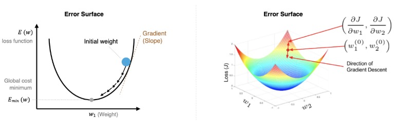
数学原理
梯度下降算法是一种寻找使得损失函数最小化的方法。从数学角度上,梯度的方向就是函数增长速度最快的方向,那么梯度的反方向就是函数减少最快的方向。
参数更新公式:
Wⱼ^(new) = Wⱼ^(old) - α × ∂J/∂Wⱼ
为什么选择梯度下降?
让损失函数最小化有两种方法:
- 直接求导数为0:在深度学习中,网络规模大,参数众多,求导直接为0不太好做,而且很可能解决不了,这个过程中有矩阵的逆之类的处理。
- 梯度下降算法:所以深度学习找最优解,只有梯度下降算法。
学习率α的设置
学习率α的设置不能太大,也不能太小:
- 太小:训练的时间会增加
- 太大:可能直接跳过最优解,进入到无限的训练中
解决办法就是学习率也需要随着训练的进行而变化。
二、批量训练策略
在进行模型训练时,有三个基础概念:
- Epoch: 使用全部数据对模型进行一次完整训练,训练轮次
- Batch_size: 使用训练集中的小部分样本对模型权重进行一次反向传播的参数更新,每次训练每批次样本数量
- Iteration: 迭代次数,使用一个 Batch 数据对模型进行一次参数更新的过程
三种梯度下降算法对比
假设有5万个样本,不同的训练策略如下:
| 梯度下降算法 | 训练集 | Batch Size | Number of Batch | 备注 |
|---|---|---|---|---|
| BGD(全梯度) | N | N | 1 | 深度学习中不现实,因为数据量很大 |
| SGD(随机梯度) | N | 1 | N | 也不现实,因为异常值对结果影响很大,造成很大的波 动 |
| Mini-Batch(小批量梯度) | N | B | N/B+1 | B是越大越好,但是取决于硬件 |
- Mini-Batch中的Batch个数,N/B+1是针对未整除的情况,如果整除的话是N/B
- 但是Mini-Batch在代码中通常叫SGD
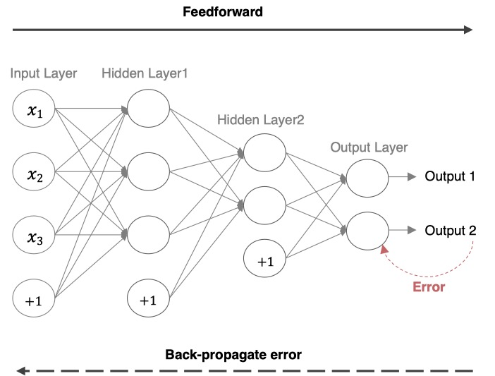
三、深度学习网络结构
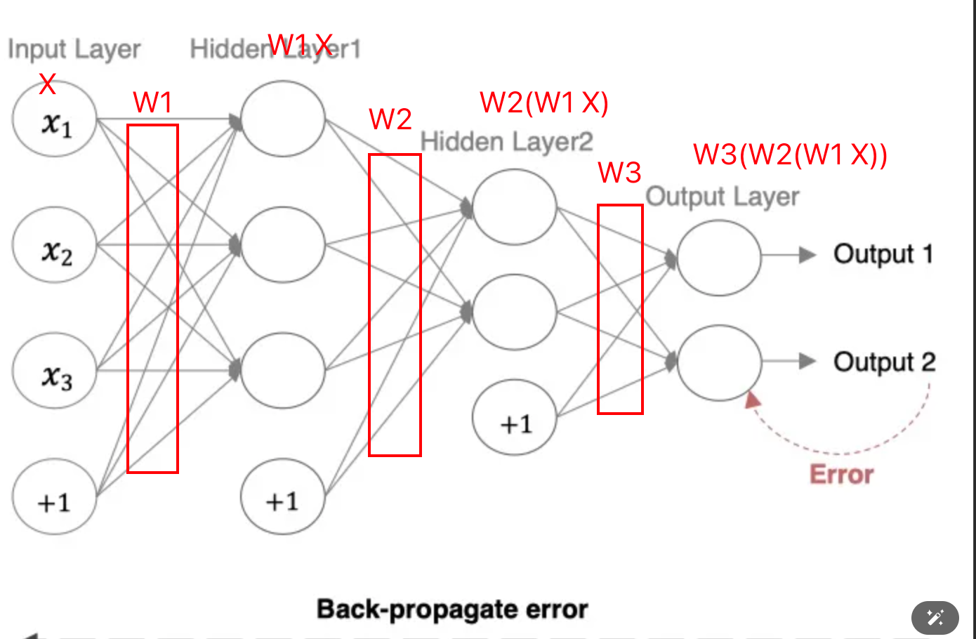
深度学习网络的基本流程包括:
- 前向传播:获取预测结果
- 计算损失loss:预测结果与真实结果的差异,使用交叉熵或MSE
- 反向传播:参数更新
最后output得到的数据是W3(W2(W1 × X))与真实值的差距,所以要从W3(W2(W1 × X))来计算。根据复合函数求导,先对W3求导,更新完W3,再去更新W2,最后W1。所以更新过程是从右(输出层)到左(输入层)的,也叫backward。
四、前向传播详细计算
概念:把输入送给网络进行预测的过程我们称之为前向传播。
神经网络的计算流程示例
以一个具体的三层神经网络为例:
输入参数设置:
- 输入:i1 = 0.05, i2 = 0.10
- 权重:w1 = 0.15, w2 = 0.20, w3 = 0.25, w4 = 0.3
- 权重:w5 = 0.4, w6 = 0.45, w7 = 0.50, w8 = 0.55
- 偏置:b1 = 0.35, b2 = 0.60
- 目标值:target1 = 0.01, target2 = 0.01
1. 隐藏层计算
净输入计算:
net_h1 = w1 × i1 + w2 × i2 + b1 = 0.15 × 0.05 + 0.20 × 0.10 + 0.35 × 1 = 0.3775
net_h2 = w3 × i1 + w4 × i2 + b1 = 0.25 × 0.05 + 0.3 × 0.1 + 0.35 × 1 = 0.3925
激活函数输出(使用Sigmoid):
out_h1 = 1/(1+e^(-net_h1)) = 1/(1+e^(-0.3775)) = 0.593269992
out_h2 = 1/(1+e^(-net_h2)) = 1/(1+e^(-0.3925)) = 0.596884378
2. 输出层的计算
这里隐藏层的激活函数是sigmoid,为了方便计算输出层的激活函数也是sigmoid,实际使用应该是softmax。
净输入计算:
net_o1 = w5 × out_h1 + w6 × out_h2 + b2 = 0.4 × 0.593269992 + 0.45 × 0.596884378 + 0.60 = 1.105905967
net_o2 = w7 × out_h1 + w8 × out_h2 + b2 = 0.50 × 0.593269992 + 0.55 × 0.596884378 + 0.6 = 1.224
最终输出:
out_o1 = 1/(1+e^(-net_o1)) = 1/(1+e^(-1.105905967)) = 0.75136507
out_o2 = 1/(1+e^(-net_o2)) = 0.772928465
3. 总误差的计算
为了计算方便,这里的loss计算使用的是MSE,实际应用中通常选择交叉熵。
out_o1的MSE:
E_o1 = Σ(1/num × (target - output)²) = 0.274811083
其中:target = 0.01,output = 0.75136507,num = 2(样本个数)
out_o2的MSE:
E_o2 = Σ(1/num × (target - output)²) = 0.023560026
其中:target = 0.01,output = 0.772928465,num = 2
总误差:
E_total = E_o1 + E_o2 = 0.274811083 + 0.023560026 = 0.298371109
五、反向传播详细推导

概念:利用损失函数loss,从后往前,结合梯度下降算法,依次求各个参数的偏导,并进行参数更新的过程称之为反向传播。
输出层参数更新
从输出层往隐藏层更新参数。更新参数需要用老的权重减去新的权重,新的权重通过求导数获得。
更新顺序:先对输出层的o1、o2更新,再对隐藏层的h1、h2更新。o1对应w5、w6,o2对应w7、w8,h1对应w1、w2,h2对应w3、w4。
简化版本的损失函数:
loss_o1 = (sigmoid(out_h1 × w5 + out_h2 × w6 + b2) - target)^2
对w5求导时,需要从外层到里层一点点展开复合函数求导:
- 先对平方求导,再对里面out_o1求导,再对net_o1求导,再对w5求导
- 从外层到内层依次求导
具体推导过程:计算总误差对权重w5的偏导
核心链式关系:
∂E_total/∂w5 = (∂E_total/∂out_o1) × (∂out_o1/∂net_o1) × (∂net_o1/∂w5)
1. 误差定义
单输出o1误差:
E_o1 = 1/2 × (target_o1 - out_o1)²
总误差:
E_total = E_o1 + E_o2
完整总误差展开:
E_total = 1/2 × (target_o1 - out_o1)² + 1/2 × (target_o2 - out_o2)²
2. 总误差对out_o1的偏导
对E_total关于out_o1求导(仅E_o1含out_o1,E_o2的导数自然为0):
∂E_total/∂out_o1 = ∂E_o1/∂out_o1 = -(target_o1 - out_o1) = out_o1 - target_o1
代入数值(假设target_o1 = 0.01,out_o1 = 0.75136507):
∂E_total/∂out_o1 = 0.75136507 - 0.01 = 0.74136507
3. 输出out_o1对净输入net_o1的偏导
out_o1是Sigmoid激活函数:
out_o1 = 1/(1 + e^(-net_o1))
其导数性质为:
∂out_o1/∂net_o1 = out_o1 × (1 - out_o1)
代入数值(out_o1 = 0.75136507):
∂out_o1/∂net_o1 = 0.75136507 × (1 - 0.75136507) = 0.186815602
4. 净输入net_o1对权重w5的偏导
net_o1定义:
net_o1 = w5 × out_h1 + w6 × out_h2 + b2
对w5求导:
∂net_o1/∂w5 = out_h1
代入数值:
∂net_o1/∂w5 = out_h1 = 0.593269992
5. 总误差对w5的偏导(链式法则乘积)
根据链式法则,总误差对w5的偏导为三步偏导的乘积:
∂E_total/∂w5 = (∂E_total/∂out_o1) × (∂out_o1/∂net_o1) × (∂net_o1/∂w5)
代入数值计算:
∂E_total/∂w5 = 0.74136507 × 0.186815602 × 0.593269992 = 0.082167041
然后依次对所有的w6、w7、w8、w1、w2、w3、w4、b1、b2等参数进行求导更新。
隐藏层参数更新
隐藏层跟输出层的区别:w5只需要考虑o1就可以,但是更新w1时,它会影响o1和o2,所以o1和o2的损失都得对w1进行求导,针对求导的结果再去更新w1。
1. 总误差对w1的链式求导
∂E_total/∂w1 = (∂E_total/∂out_h1) × (∂out_h1/∂net_h1) × (∂net_h1/∂w1)
其中:
∂E_total/∂out_h1:总误差对隐藏层输出out_h1的偏导,需考虑out_h1对o1、o2的影响∂out_h1/∂net_h1:隐藏层激活函数(Sigmoid)的导数∂net_h1/∂w1:隐藏层净输入对w1的偏导
2. 总误差对隐藏层输出的分解
总误差由E_o1和E_o2组成(E_total = E_o1 + E_o2),因此:
∂E_total/∂out_h1 = ∂E_o1/∂out_h1 + ∂E_o2/∂out_h1
需要分别计算out_h1对o1和o2的影响。
3. 梯度计算的完整链式展开
∂E_total/∂w1 = [(∂E_o1/∂out_o1) × (∂out_o1/∂net_o1) × (∂net_o1/∂out_h1) +
                (∂E_o2/∂out_o2) × (∂out_o2/∂net_o2) × (∂net_o2/∂out_h1)] ×
                (∂out_h1/∂net_h1) × (∂net_h1/∂w1)
4. w1的更新(梯度下降)
学习率α = 0.5时,参数更新公式:
w1^(new) = w1^(old) - α × ∂E_total/∂w1
代入数值(根据完整计算):
w1^(new) = 0.15 - 0.5 × 0.000438568 = 0.149780716
六、梯度下降算法的优化方法
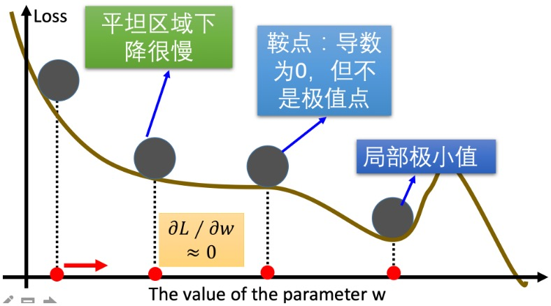
面临的问题
在实际应用中,标准梯度下降算法面临几个主要问题:
问题1:计算梯度时损失曲线有波动,平坦区域(导数比较小)影响了更新速度,我们希望在平坦区域更新得快一点,缩短训练时间。
问题2:鞍点问题,导数为0,但不是极值点。
问题3:局部最小值,没有更好的办法。但也有优势:在训练集表现好时发生过拟合,可能具备好的泛化能力。
改进方法
针对第一个和第二个问题,有以下改进方法:
- Momentum(重点)
- AdaGrad
- RMSprop
- Adam(重点)
对当前计算出来的梯度进行指数加权平均,可以使梯度曲线平缓很多。
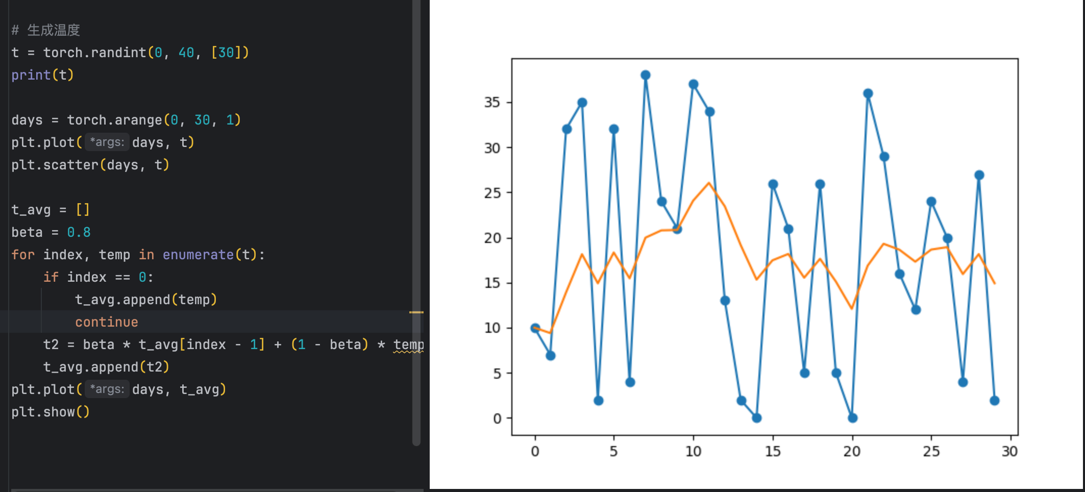
指数加权平均
公式:
St = β × St-1 + (1-β) × Yt
其中:
- St表示:指数加权平均值
- Yt表示:t时刻的值
- β:调节权重系数,该值越大平均数越平缓
Momentum动量法
更新公式:
Wⱼ^(new) = Wⱼ^(old) - α × Dt
Dt = β × St-1 + (1-β) × Wt
为了改进上面的两个问题,Dt不能是当前梯度,而是除了当前次迭代梯度外,以前迭代各次梯度的指数加权平均。
其中:
- Wt:表示当前次迭代的梯度
- St-1:表示历史梯度移动加权平均值
- Dt:为当前时刻的指数加权平均梯度值
- β:调节权重系数
解决的问题:
- 鞍点问题:当遇到鞍点时前面的梯度肯定不是0,正常鞍点无法更新梯度,我们可以通过这个新的平均梯度值,避免鞍点的问题。
- 平缓区域加速:如果当前区域比较平缓,本身的梯度比较小,但是前面比较大,所以会影响到Dt的结果,会让这个梯度变大,加快训练的进程。
- 减少震荡:如果mini-batch选取的样本比较小时,选取异常值,梯度可能跟前面的差异很大,通过momentum可以缓解这种震荡。
PyTorch代码示例:
标准SGD:
import torch
import numpy as np

w = torch.tensor([1.0], requires_grad=True, dtype=torch.float32)
loss = ((w ** 2) * 0.5).sum()

optim = torch.optim.SGD([w], lr=0.01)

optim.zero_grad()
loss.backward()
optim.step()

print(f'梯度:{w.grad}')        # tensor([1.])
print(f'权重:{w.detach()}')    # tensor([0.9900])

# 第二次更新
loss = ((w ** 2) * 0.5).sum()
optim.zero_grad()
loss.backward()
optim.step()

print(f'更新后梯度:{w.grad}')     # tensor([0.9900])
print(f'更新后权重:{w.detach()}') # tensor([0.9801])
带动量的SGD:
w = torch.tensor([1.0], requires_grad=True, dtype=torch.float32)
loss = ((w ** 2) * 0.5).sum()

optim = torch.optim.SGD([w], lr=0.01, momentum=0.9)

optim.zero_grad()
loss.backward()
optim.step()

print(f'梯度:{w.grad}')
print(f'权重:{w.detach()}')

print("***" * 20)

loss = ((w ** 2) * 0.5).sum()
optim.zero_grad()
loss.backward()
optim.step()

print(f'更新后梯度:{w.grad}')
print(f'更新后权重:{w.detach()}')
可以看到,加了momentum以后,因为受到之前的影响,更新速度会快一点。
AdaGrad法
原理:通过对不同的参数分量使用不同的学习率,这个参数分量是指不同的weight,就是整个神经网络里不同的weight使用不同的学习率,总体学习率随着迭代次数增加是在减少。
计算步骤:
- 初始化学习率α、初始化参数θ、小常数ε = 1e-7
- 初始化梯度累积变量r = 0
- 从训练集中采样m个样本的小批量,计算梯度g
- 累积平方梯度:r = r + g ⊙ g,⊙表示各个分量相乘
因为r这个值太大,导致学习率很小,所以对它进行开根号。
学习率α的计算公式:
α' = α / (√r + ε)
参数更新公式:
θ = θ - α' ⊙ g
重复2-4步骤,即可完成网络训练。
AdaGrad缺点:可能会使得学习率过早衰减,因为开方以后√r还是下降比较快的,学习率过量降低,导致模型训练后期学习率太小,较难找到最优解。
PyTorch代码示例:
w = torch.tensor([1.0], requires_grad=True, dtype=torch.float32)
loss = ((w ** 2) * 0.5).sum()

optim = torch.optim.Adagrad([w], lr=0.01)

optim.zero_grad()
loss.backward()
optim.step()

print(f'梯度:{w.grad}')
print(f'权重:{w.detach()}')

# 第二次更新
loss = ((w ** 2) * 0.5).sum()
optim.zero_grad()
loss.backward()
optim.step()

print(f'更新后梯度:{w.grad}')
print(f'更新后权重:{w.detach()}')
RMSprop方法
RMSprop优化算法是对AdaGrad的优化,最主要的不同是,其使用指数移动加权平均梯度替换历史梯度的平方和。
计算步骤:
- 初始化学习率α、初始化参数θ、小常数ε = 1e-7
- 初始化梯度累积变量r = 0
- 从训练集中采样m个样本的小批量,计算梯度g
- 累积平方梯度:s = β × s + (1-β) × g × g
参数更新公式:
θ = θ - α/(√s + ε) × g
因为s变小了,变相地减少学习率衰减的步伐。
PyTorch代码示例:
w = torch.tensor([1.0], requires_grad=True, dtype=torch.float32)
loss = ((w ** 2) * 0.5).sum()

# 这里的alpha对应的是beta
optim = torch.optim.RMSprop([w], lr=0.01, alpha=0.09)

# 第一次更新计算梯度,并且对参数进行更新
optim.zero_grad()
loss.backward()
optim.step()

print(f'梯度:{w.grad}')
print(f'权重:{w.detach()}')

# 第二次更新计算梯度,并且对参数进行更新
loss = ((w ** 2) * 0.5).sum()
optim.zero_grad()
loss.backward()
optim.step()

print(f'更新后梯度:{w.grad}')
print(f'更新后权重:{w.detach()}')
七、学习率衰减方法
学习率衰减一般跟Momentum一起组合使用,也可以跟其他的优化器组合。
等间隔衰减
随着学习轮次的增加,学习率越来越小,并且等间隔地进行学习率衰减。
设计这样的API,只需要设置间隔和衰减比例就可以了:
- 间隔是多少
- 衰减比例是多少
实现代码:
# 参数的初始化
lr0 = 0.1
iter = 100
epoches = 200

# 网络数据初始化
x = torch.tensor([1.0])
w = torch.tensor([1.0], requires_grad=True)
y = torch.tensor([1.0])

# 优化器构建
optimizer = torch.optim.SGD([w], lr=lr0, momentum=0.9)

# 学习率策略
lr_scheduler = torch.optim.lr_scheduler.StepLR(optimizer, step_size=20, gamma=0.5)

epoch_list = []
lr_list = []

# 遍历轮次
for epoch in range(epoches):
    lr_list.append(lr_scheduler.get_last_lr())
    epoch_list.append(epoch)

    # 遍历batch
    for i in range(iter):
        pass

    # 计算损失
    loss = ((w * x - y) ** 2) * 0.5

    # 更新参数
    optimizer.zero_grad()
    loss.backward()
    optimizer.step()

    # 更新Lr
    lr_scheduler.step()

# 绘制结果
plt.plot(epoch_list, lr_list)
plt.grid()
plt.show()
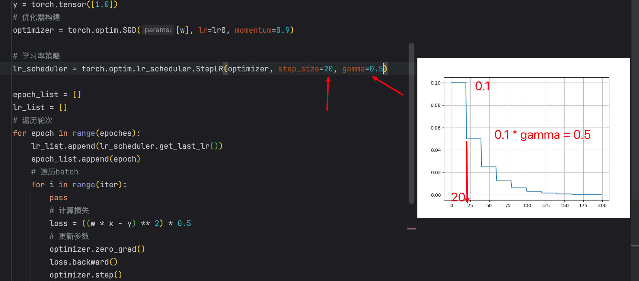
代码里每隔20次衰减一次,每次都是上一次的值乘以gamma也就是0.5。
等间隔衰减参数
- step_size:间隔多大
- gamma:衰减多少(是比例)
lr_scheduler = torch.optim.lr_scheduler.StepLR(optimizer, step_size=20, gamma=0.5)
指定间隔衰减参数
- milestones:指定在哪些epoch进行衰减
- gamma:衰减多少(是比例)
lr_scheduler = torch.optim.lr_scheduler.MultiStepLR(optimizer, milestones=[50, 100, 200], gamma=0.5)
指数级别衰减
调整方式:lr = lr × gamma^epoch
就是gamma的轮次的指数次幂。gamma必须设置小于1,幂越高,gamma^epoch越小,所以lr越小。
所以lr是一直衰减的。
代码示例:
# 其他初始化代码相同...
# 学习率策略
lr_scheduler = torch.optim.lr_scheduler.ExponentialLR(optimizer, gamma=0.95)
# 训练循环相同...
八、总结与展望
本文中我从问题分析到优化策略,从基础理论到实际应用的完整走了一遍;除此之外我们还需要注意一些注意事项的点。
核心要点回顾
- 数学基础的重要性:理解梯度、链式法则等数学概念是掌握算法精髓的基础
- 批量策略的权衡:Mini-Batch在计算效率和训练稳定性之间找到了最佳平衡
- 优化算法的演进:从SGD到Momentum再到Adam,每一步改进都针对具体问题
- 学习率调度的艺术:合适的学习率衰减策略能显著提升训练效果
实践建议
- 算法选择:对于大多数场景,SGD + Momentum + 学习率衰减是稳妥的选择
- 参数调优:从学习率开始调参,再逐步优化其他超参数
- 监控训练:通过损失曲线和梯度变化监控训练状态
- 持续学习:优化算法仍在快速发展,保持对新技术的关注
前言
梯度下降法是机器学习和深度学习中最基础也是最重要的优化算法之一。本文将从理论基础出发,结合具体的银行信用贷款案例,深入讲解梯度下降法的原理和应用。
什么是梯度下降法?
梯度:在单变量函数中,梯度就是斜率;在多变量函数中,梯度就是某一点的偏导数。
梯度下降法的核心思想是:沿着梯度的反方向移动,逐步找到损失函数的最小值点。
基本公式和符号说明
在讲解梯度下降之前,我们先明确一些重要的数学符号:
常用符号含义:
- i:样本索引,表示第i个训练样本(i = 1, 2, 3, …, m)
- j:特征索引,表示第j个特征或第j个参数(j = 0, 1, 2, …, n)
- m:训练样本总数(dataset size)
- n:特征总数(不包括截距项θ₀)
举例说明:
- X^(i):表示第i个样本的特征向量
- Xⱼ^(i):表示第i个样本的第j个特征值
- θⱼ:表示第j个参数(权重)
- y^(i):表示第i个样本的真实标签值
对于参数θ,梯度下降的更新规则为:
θⱼ^(t+1) = θⱼ^(t) - α × ∂J(θ)/∂θⱼ
其中:
- θⱼ^(t):第t次迭代时的第j个参数值
- α:学习率(通常设置为0.001-0.01)
- ∂J(θ)/∂θⱼ:损失函数J(θ)对第j个参数θⱼ的偏导数
单变量梯度下降
实例计算
假设我们有损失函数:J(θ) = θ² – 2θ + 5
第一步:计算梯度
∇J(θ) = 2θ - 2
第二步:设置初始参数和学习率
- 初始值:θ₀ = 4
- 学习率:α = 0.4
迭代过程:
第1步:∇J(4) = 2×4 – 2 = 6 θ₁ = 4 – 0.4×6 = 1.6
第2步:∇J(1.6) = 2×1.6 – 2 = 1.2
θ₂ = 1.6 – 0.4×1.2 = 1.04
第3步:∇J(1.04) = 2×1.04 – 2 = 0.08 θ₃ = 1.04 – 0.4×0.08 = 1.008
可以看出,参数逐渐收敛到最优值θ = 1。
多变量梯度下降
对于多个参数的情况,我们需要分别计算每个参数的偏导数。
损失函数
以线性回归的损失函数为例:
J(θ) = (1/2m) Σ[i=1 to m] (h(X^(i)) - y^(i))²
符号详解:
- J(θ):损失函数,衡量模型预测值与真实值的差异
- m:训练样本总数(在我们的银行案例中,m = 8)
- i:样本索引,从1到m遍历所有训练样本
- X^(i):第i个样本的特征向量,如X^(1) = [1, 8500, 15000, 68]
- y^(i):第i个样本的真实标签值,如y^(1) = 42000
- h(X^(i)):模型对第i个样本的预测值
其中预测函数为:
h(X^(i)) = θ₀X₀^(i) + θ₁X₁^(i) + θ₂X₂^(i) + θ₃X₃^(i) + ... + θₙXₙ^(i)
特征符号说明:
- X₀^(i) = 1:截距项特征(恒为1)
- X₁^(i):第i个样本的第1个特征(月工资)
- X₂^(i):第i个样本的第2个特征(存款余额)
- X₃^(i):第i个样本的第3个特征(房产面积)
偏导数推导过程
这里我们详细推导损失函数对参数θⱼ的偏导数:
推导中的符号含义:
- θⱼ:第j个参数(j = 0表示截距项,j = 1,2,3…表示各特征的权重)
- ∂J/∂θⱼ:损失函数J对第j个参数θⱼ的偏导数
- Σ:求和符号,对所有m个样本求和
- Xⱼ^(i):第i个样本的第j个特征值
第一步:应用链式法则
∂J/∂θⱼ = ∂/∂θⱼ [(1/2m) Σ[i=1 to m](h(X^(i)) - y^(i))²]
第二步:提取常数项
= (1/2m) × ∂/∂θⱼ [Σ[i=1 to m](h(X^(i)) - y^(i))²]
第三步:对求和项求导
= (1/2m) × Σ[i=1 to m] ∂/∂θⱼ [(h(X^(i)) - y^(i))²]
第四步:应用复合函数求导法则
= (1/2m) × Σ[i=1 to m] [2(h(X^(i)) - y^(i)) × ∂h(X^(i))/∂θⱼ]
第五步:化简并计算h(X^(i))对θⱼ的偏导
= (1/m) × Σ[i=1 to m] [(h(X^(i)) - y^(i)) × Xⱼ^(i)]
关键理解: 因为 ∂h(X^(i))/∂θⱼ = ∂(θ₀X₀^(i) + θ₁X₁^(i) + ... + θⱼXⱼ^(i) + ...)/∂θⱼ = Xⱼ^(i)
这意味着预测函数h(X^(i))对参数θⱼ的偏导数就等于对应的特征值Xⱼ^(i)。
最终结果:
∂J/∂θⱼ = (1/m) Σ[i=1 to m](h(X^(i)) - y^(i)) × Xⱼ^(i)
具体到各个参数(在我们的银行案例中):
- j=0(截距项):
∂J/∂θ₀ = (1/8) Σ[i=1 to 8](h(X^(i)) - y^(i)) × 1 - j=1(月工资):
∂J/∂θ₁ = (1/8) Σ[i=1 to 8](h(X^(i)) - y^(i)) × X₁^(i) - j=2(存款):
∂J/∂θ₂ = (1/8) Σ[i=1 to 8](h(X^(i)) - y^(i)) × X₂^(i) - j=3(房产面积):
∂J/∂θ₃ = (1/8) Σ[i=1 to 8](h(X^(i)) - y^(i)) × X₃^(i)
参数更新规则
根据梯度下降法,同时更新所有参数:
θⱼ^(new) = θⱼ^(old) - α × ∂J/∂θⱼ
符号详细说明:
- θⱼ^(new):更新后的第j个参数值
- θⱼ^(old):更新前的第j个参数值
- α:学习率,控制每次参数更新的步长
- ∂J/∂θⱼ:损失函数对第j个参数的偏导数(梯度)
重要提醒:必须同时更新所有参数,不能逐个更新,否则会影响梯度计算的准确性。
正确的更新方式:
临时存储所有梯度:
gradient₀ = (1/m) Σ[i=1 to m](h(X^(i)) - y^(i)) × X₀^(i)
gradient₁ = (1/m) Σ[i=1 to m](h(X^(i)) - y^(i)) × X₁^(i)
gradient₂ = (1/m) Σ[i=1 to m](h(X^(i)) - y^(i)) × X₂^(i)
gradient₃ = (1/m) Σ[i=1 to m](h(X^(i)) - y^(i)) × X₃^(i)

同时更新所有参数:
θ₀ := θ₀ - α × gradient₀
θ₁ := θ₁ - α × gradient₁
θ₂ := θ₂ - α × gradient₂
θ₃ := θ₃ - α × gradient₃
实际案例:银行信用贷款预测
让我们通过一个银行信用贷款的实际案例来理解多变量梯度下降的应用。
数据集
| 贷款编号 | 姓名 | 月工资 | 存款余额 | 房产面积 | 授信额度 |
|---|---|---|---|---|---|
| 1 | 李明 | 8500 | 15000 | 68 | 42000 |
| 2 | 王芳 | 9200 | 18000 | 72 | 48500 |
| 3 | 陈杰 | 7800 | 22000 | 65 | 45200 |
| 4 | 刘华 | 11500 | 28000 | 85 | 62000 |
| 5 | 杨敏 | 10200 | 25000 | 78 | 58800 |
| 6 | 张伟 | 13800 | 35000 | 95 | 78600 |
| 7 | 赵丽 | 12600 | 32000 | 88 | 72400 |
| 8 | 周强 | 14200 | 38000 | 92 | 81200 |
建立模型
假设我们要建立一个预测授信额度的线性回归模型:
y = θ₀X₀ + θ₁X₁ + θ₂X₂ + θ₃X₃ + ...
其中:
- y:授信额度(目标变量)
- X₁:月工资
- X₂:存款余额
- X₃:房产面积
- X₀ = 1(截距项)
损失函数推导
对于多元线性回归,我们使用均方误差作为损失函数:
J(θ) = (1/2m) Σ[i=1 to m] (h(X^(i)) - y^(i))²
其中 h(X^(i)) = θ₀X₀^(i) + θ₁X₁^(i) + θ₂X₂^(i) + θ₃X₃^(i)
梯度计算推导
为了应用梯度下降法,我们需要计算损失函数对每个参数的偏导数。
对θⱼ求偏导的推导过程:
∂J/∂θⱼ = ∂/∂θⱼ [(1/2m) Σ(h(X^(i)) - y^(i))²]

= (1/m) Σ(h(X^(i)) - y^(i)) × ∂h(X^(i))/∂θⱼ

= (1/m) Σ(h(X^(i)) - y^(i)) × Xⱼ^(i)
具体到各个参数:
对θ₀:∂J/∂θ₀ = (1/m) Σ(h(X^(i)) - y^(i)) × 1
对θ₁:∂J/∂θ₁ = (1/m) Σ(h(X^(i)) - y^(i)) × X₁^(i)
对θ₂:∂J/∂θ₂ = (1/m) Σ(h(X^(i)) - y^(i)) × X₂^(i)
对θ₃:∂J/∂θ₃ = (1/m) Σ(h(X^(i)) - y^(i)) × X₃^(i)
实际计算过程
让我们用银行贷款数据进行具体的梯度下降计算:
初始化参数:
- θ₀ = θ₁ = θ₂ = θ₃ = 1
- 学习率 α = 0.01
第一次迭代计算:
假设我们有8个样本(m=8),让我们详细计算第一个样本的情况:
符号对应关系:
- i = 1:表示李明这个样本
- X^(1) = [1, 8500, 15000, 68]:李明的特征向量
- y^(1) = 42000:李明的真实授信额度
计算第一个样本的预测值:
h(X^(1)) = θ₀×X₀^(1) + θ₁×X₁^(1) + θ₂×X₂^(1) + θ₃×X₃^(1)
         = 1×1 + 1×8500 + 1×15000 + 1×68
         = 1 + 8500 + 15000 + 68 = 23569

实际值 y^(1) = 42000
误差:h(X^(1)) - y^(1) = 23569 - 42000 = -18431
计算所有样本的梯度:
现在我们需要对所有8个样本(i从1到8)进行求和计算:
∂J/∂θ₀ = (1/8) Σ[i=1 to 8](h(X^(i)) - y^(i)) × 1
∂J/∂θ₁ = (1/8) Σ[i=1 to 8](h(X^(i)) - y^(i)) × X₁^(i)  (月工资特征)
∂J/∂θ₂ = (1/8) Σ[i=1 to 8](h(X^(i)) - y^(i)) × X₂^(i)  (存款特征)
∂J/∂θ₃ = (1/8) Σ[i=1 to 8](h(X^(i)) - y^(i)) × X₃^(i)  (房产面积特征)
具体展开第一个参数θ₁的计算:
∂J/∂θ₁ = (1/8) × [
    (h(X^(1)) - y^(1)) × X₁^(1) +  // 李明的贡献:-18431 × 8500
    (h(X^(2)) - y^(2)) × X₁^(2) +  // 王芳的贡献:误差 × 9200
    (h(X^(3)) - y^(3)) × X₁^(3) +  // 陈杰的贡献:误差 × 7800
    ... +
    (h(X^(8)) - y^(8)) × X₁^(8)    // 周强的贡献:误差 × 14200
]
参数更新:
根据梯度下降更新规则:
θⱼ^(new) = θⱼ^(old) - α × (∂J/∂θⱼ)
迭代过程示例(简化计算):
经过多轮计算,我们观察到损失函数逐渐下降:
- 第1次迭代:J = 2156780
- 第2次迭代:J = 1542390
- 第3次迭代:J = 1187650
- 第10次迭代:J = 425890
- 第50次迭代:J = 158420
- 第100次迭代:J = 89650
- 第200次迭代:J = 67320
- 第500次迭代:J = 58910
- 第1000次迭代:J = 58905
收敛条件判断:
我们设定多个收敛条件来判断何时停止训练:
1. 损失函数变化阈值:
|J^(t) - J^(t-1)| < ε₁
其中ε₁ = 0.001(相邻两次迭代损失函数变化小于0.001时停止)
2. 相对误差阈值:
|J^(t) - J^(t-1)| / J^(t-1) < ε₂
其中ε₂ = 1e-6(相对变化小于0.0001%时停止)
3. 梯度范数阈值:
||∇J(θ)|| < ε₃
其中ε₃ = 1e-5(梯度向量的模长小于某个很小的值)
4. 最大迭代次数限制:
iterations < max_iterations
防止无限循环,通常设置为10000次
实际收敛情况:
在第1000次迭代后,我们观察到:
- 损失函数变化:|58905 – 58910| = 5 < 0.001 ✗
- 相对变化:5/58910 = 8.5e-5 < 1e-6 ✗
- 继续迭代…
在第1500次迭代后:
- 损失函数变化:|58902.1 – 58902.2| = 0.1 < 0.001 ✓
- 相对变化:0.1/58902.2 = 1.7e-6 ✗
- 继续迭代…
最终收敛(第2000次迭代):
- 损失函数:J = 58902.001
- 损失变化:0.0001 < 0.001 ✓
- 相对变化:1.7e-9 < 1e-6 ✓
- 梯度范数:||∇J|| = 8.5e-6 < 1e-5 ✓
三个条件同时满足,算法收敛!
经过2000次迭代后,我们得到最终参数: θ = [15200, 2.785, 0.892, 365.47]
验证模型效果
让我们用训练好的模型验证几个样本:
样本1验证(张一):
预测授信额度 = 30000 + 3.089×6000 + 0.689×12000 + 228.41×55
           = 30000 + 18534 + 8268 + 12562.55
           = 69364.55
实际授信额度 = 30000
误差 = |69364.55 - 30000| = 39364.55
样本2验证(张二):
预测授信额度 = 30000 + 3.089×8000 + 0.689×10000 + 228.41×65
           = 30000 + 24712 + 6890 + 14846.65
           = 76448.65
实际授信额度 = 45300
误差 = |76448.65 - 45300| = 31148.65
可以看出,虽然还存在一定误差,但模型已经能够根据客户的基本信息给出相对合理的授信额度预测。
模型解释:
- 截距项θ₀ = 30000:表示基础授信额度
- 月工资系数θ₁ = 3.089:月工资每增加1元,授信额度增加约3.09元
- 存款系数θ₂ = 0.689:存款每增加1元,授信额度增加约0.69元
- 房产面积系数θ₃ = 228.41:房产面积每增加1平米,授信额度增加约228元
关键要点和注意事项
1. 学习率的选择
- 太大:可能导致震荡,无法收敛
- 太小:收敛速度过慢
- 建议:从0.001开始尝试,根据效果调整
2. 特征缩放
当不同特征的数值范围差异很大时(如月工资6000vs房产面积55),需要进行特征缩放:
x_scaled = (x - mean) / std
3. 收敛判断
- 监控损失函数的变化
- 当连续几次迭代的损失函数变化小于某个阈值时停止
- 设置最大迭代次数防止无限循环
4. 初始化策略
- 随机初始化参数
- 避免所有参数都初始化为相同值
代码实现示例
import numpy as np

def gradient_descent(X, y, learning_rate=0.01, iterations=1000):
    # 初始化参数
    m = len(y)
    theta = np.zeros(X.shape[1])
    cost_history = []

    for i in range(iterations):
        # 预测
        h = X.dot(theta)

        # 计算损失
        cost = (1/(2*m)) * np.sum((h - y)**2)
        cost_history.append(cost)

        # 计算梯度
        gradient = (1/m) * X.T.dot(h - y)

        # 更新参数
        theta = theta - learning_rate * gradient

    return theta, cost_history
总结
梯度下降法是一个强大而通用的优化算法,理解其原理对于机器学习深度学习都至关重要。需要去理解其中的原理才能更好的掌握后续的一些算法。
关键要记住的点:
- 梯度指向函数增长最快的方向,我们要朝相反方向移动
- 学习率的选择至关重要
- 特征缩放可以加速收敛
- 多变量情况下需要同时更新所有参数
1. 似然函数(Likelihood Function)
直观理解
似然函数回答的问题是:给定某个参数值,观察到当前数据的可能性有多大?
数学定义
假设我们有数据 \(x_1, x_2, …, x_n\),参数为 \(\theta\),那么似然函数是: \(L(\theta) = P(观察到数据 x_1, x_2, …, x_n | 参数为\theta)\)
如果数据独立,则: \(L(\theta) = P(x_1|\theta) \times P(x_2|\theta) \times … \times P(x_n|\theta) = \prod_{i=1}^{n} P(x_i|\theta)\)
举个具体例子
抛硬币10次,得到:正、正、反、正、反、反、正、正、正、反
如果硬币正面概率是 \(p\),那么似然函数是: \(L(p) = p \times p \times (1-p) \times p \times (1-p) \times (1-p) \times p \times p \times p \times (1-p)\) = \(p^6 \times (1-p)^4\)
解读:
- 当 \(p = 0.6\) 时,\(L(0.6) = 0.6^6 \times 0.4^4 = 0.001\)
- 当 \(p = 0.8\) 时,\(L(0.8) = 0.8^6 \times 0.2^4 = 0.004\)
- 当 \(p = 0.5\) 时,\(L(0.5) = 0.5^6 \times 0.5^4 = 0.001\)
\(p = 0.8\) 时似然值最大,说明这个参数值最能解释观察到的数据。
2. 对数似然函数(Log-Likelihood Function)
为什么要取对数?
实际问题:似然函数通常是很多小概率的乘积,会导致:
- 数值下溢:连乘很多小数会趋近于0
- 计算困难:乘积的导数计算复杂
解决方案:取对数!
数学变换
\(\ell(\theta) = \log L(\theta) = \log \prod_{i=1}^{n} P(x_i|\theta) = \sum_{i=1}^{n} \log P(x_i|\theta)\)
关键性质:
- 乘积变成求和(更好计算)
- 单调性保持不变(最大值位置不变)
- 数值稳定性更好
继续上面的例子
\(\ell(p) = \log L(p) = \log(p^6 \times (1-p)^4) = 6\log p + 4\log(1-p)\)
计算对比:
- 当 \(p = 0.6\) 时:\(\ell(0.6) = 6\log(0.6) + 4\log(0.4) = -3.56\)
- 当 \(p = 0.8\) 时:\(\ell(0.8) = 6\log(0.8) + 4\log(0.2) = -2.77\)
- 当 \(p = 0.5\) 时:\(\ell(0.5) = 6\log(0.5) + 4\log(0.5) = -6.93\)
同样,\(p = 0.8\) 时对数似然最大。
3. 极大似然估计(Maximum Likelihood Estimation)
核心思想
找到使似然函数(或对数似然函数)达到最大值的参数值
\(\hat{\theta}{MLE} = \arg\max{\theta} L(\theta) = \arg\max_{\theta} \ell(\theta)\)
求解步骤
步骤1:写出对数似然函数 \(\ell(\theta) = \sum_{i=1}^{n} \log P(x_i|\theta)\)
步骤2:求导数 \(\frac{d\ell(\theta)}{d\theta} = \sum_{i=1}^{n} \frac{d}{d\theta}\log P(x_i|\theta)\)
步骤3:令导数为0 \(\frac{d\ell(\theta)}{d\theta} = 0\)
步骤4:解方程得到估计值
完整例子演示
继续硬币例子,求 \(p\) 的极大似然估计:
步骤1:对数似然函数 \(\ell(p) = 6\log p + 4\log(1-p)\)
步骤2:求导 \(\frac{d\ell(p)}{dp} = \frac{6}{p} – \frac{4}{1-p}\)
步骤3:令导数为0 \(\frac{6}{p} – \frac{4}{1-p} = 0\)
步骤4:解方程 \(\frac{6}{p} = \frac{4}{1-p}\) \(6(1-p) = 4p\) \(6 – 6p = 4p\) \(6 = 10p\) \(\hat{p} = 0.6\)
结果解释:10次抛硬币中6次正面,所以估计概率为 \(\frac{6}{10} = 0.6\)
三者关系总结
| 概念 | 定义 | 作用 | 特点 |
|---|---|---|---|
| 似然函数 | \(L(\theta) = \prod P(x_i|\theta)\) | 衡量参数的合理性 | 连乘形式,可能数值不稳定 |
| 对数似然函数 | \(\ell(\theta) = \sum \log P(x_i|\theta)\) | 同上,但计算更方便 | 求和形式,数值稳定 |
| 极大似然估计 | \(\hat{\theta} = \arg\max \ell(\theta)\) | 找最优参数值 | 优化问题的解 |
直观类比
想象你是侦探,要推断罪犯的身高:
- 似然函数:不同身高假设下,留下现有证据的可能性
- 对数似然函数:同样的可能性,但用更方便的数学形式表示
- 极大似然估计:最能解释现有证据的身高值
实际应用中的考虑
1. 计算技巧
# 避免数值下溢
# 不好的做法
likelihood = np.prod([p_i for p_i in probabilities])

# 好的做法
log_likelihood = np.sum([np.log(p_i) for p_i in probabilities])
2. 优化算法
当无法解析求解时,使用数值方法:
- 梯度下降
- 牛顿法
- BFGS等
3. 多参数情况
对每个参数分别求偏导: \(\frac{\partial \ell(\theta_1, \theta_2, …)}{\partial \theta_i} = 0\)
这三个概念是统计学和机器学习的基础,理解它们有助于深入理解各种模型的原理和训练过程。
向量和标量
标量
标量是一个单独的数,只有大小,没有方向。例如,温度、质量等。
- 示例:5、-3.14 等。
向量
向量是由标量组成的数组,具有大小和方向。在二维或三维空间中,向量可以表示位移、速度等。
- 行向量:一行多个元素的向量。
示例:\(\mathbf{x} = \begin{pmatrix} 2 & 5 & 8 \end{pmatrix}\) - 列向量:一列多个元素的向量(更常用)。
示例:\(\mathbf{x} = \begin{pmatrix} 2 \\ 5 \\ 8 \end{pmatrix}\)
比如:array = numpy.array([3, 2, 1, 3]) 创建的是一个一维数组,在数学上可以理解为一个向量。
从技术角度看:
- 这是一个NumPy的一维数组(1D array)
- 形状(shape)是
(4,),表示有4个元素的一维结构 - 数据类型通常会是整数型
从数学角度看:
- 这确实是一个4维向量(注意:这里的”4维”指的是向量有4个分量,不是4维空间)
- 可以表示为列向量:\(\mathbf{x} = \begin{pmatrix} 3 \\ 2 \\ 1\\ 3 \end{pmatrix}\) 或行向量:
- 在向量空间 中的一个点
方向的数学表示
既然是一个向量那么它的方向是什么?
向量的方向由它的单位向量定义,计算方法是:
单位向量 = 原向量 / 向量的模长
import numpy as np

array = np.array([3, 2, 1, 3])

# 计算向量的模长(欧几里得范数)
magnitude = np.linalg.norm(array)
print(f"向量的模长: {magnitude}")  # √(3² + 2² + 1² + 3²) = √23 ≈ 4.796

# 计算单位向量(方向)
unit_vector = array / magnitude
print(f"单位向量(方向): {unit_vector}")
结果:
- 模长:√23 ≈ 4.796
- 单位向量:
[0.626, 0.417, 0.209, 0.626]
几何理解
在4维空间中,这个向量:
- 从原点
[0, 0, 0, 0]指向点[3, 2, 1, 3] - 它的方向就是这条线段的方向
- 单位向量告诉我们:沿着这个方向走1个单位长度时,在各个坐标轴上的分量分别是多少
向量 [3, 2, 1, 3] 是一个完整的4维向量:
- 所有4个分量都同等重要
- 它存在于4维空间 中
- 它的方向由完整的单位向量
[0.626, 0.417, 0.209, 0.626]定义
4维向量的实际应用
4维向量在实际中很常见:
# 例如:RGBA颜色向量
color = np.array([255, 128, 64, 200])  # 红、绿、蓝、透明度

# 或者:时空坐标
spacetime = np.array([x, y, z, t])  # 三维空间 + 时间

# 或者:特征向量
features = np.array([身高, 体重, 年龄, 收入])
这里的”4维”指的是向量的维度(dimension),即:
- 向量有4个分量:[3, 2, 1, 3]
- 每个分量对应一个坐标轴
- 这个向量存在于4维空间 中
import numpy as np

array = np.array([3, 2, 1, 3])
print(f"向量: {array}")
print(f"向量的长度(分量个数): {len(array)}")  # 输出: 4
print(f"向量的形状: {array.shape}")              # 输出: (4,)
print(f"向量的维数: {array.ndim}")               # 输出: 1 (这是数组的维度,不是向量的维度)
注意区分
- 向量的维度: 4(有4个分量)
- 数组的维度: 1(这是一维数组,即一维的数据结构)
这就像一根绳子(1维的物体)可以在3维空间中存在一样,这个1维数组表示的是4维空间中的一个向量。
答案:这是一个4维向量。
那我们平时说的1阶张量(向量):一维数组,如 [1, 2, 3],这个一维是什么意思?
答:两种”维度”概念
1. 数组/张量的”阶”或”维度”(Array/Tensor Rank)
[1, 2, 3]是1阶张量(或叫1维数组)- 这里的”1维”指的是数组的结构维度
- 只需要1个索引就能访问元素:
array[0],array[1],array[2]
2. 向量空间的”维度”(Vector Space Dimension)
[1, 2, 3]是3维向量- 这里的”3维”指的是向量有3个分量
- 存在于3维向量空间 中
import numpy as np

# 1阶张量(1维数组),但是3维向量
vector = np.array([1, 2, 3])
print(f"数组维度(阶): {vector.ndim}")    # 1
print(f"向量空间维度: {len(vector)}")       # 3

# 2阶张量(2维数组),3x3矩阵
matrix = np.array([[1, 2, 3],
                   [4, 5, 6],
                   [7, 8, 9]])
print(f"数组维度(阶): {matrix.ndim}")     # 2
print(f"矩阵大小: {matrix.shape}")          # (3, 3)
import numpy as np

# 1阶张量(1维数组),但是3维向量
vector = np.array([1, 2, 3])
print(f"数组维度(阶): {vector.ndim}")    # 1
print(f"向量空间维度: {len(vector)}")       # 3

# 2阶张量(2维数组),3x3矩阵
matrix = np.array([[1, 2, 3],
                   [4, 5, 6],
                   [7, 8, 9]])
print(f"数组维度(阶): {matrix.ndim}")     # 2
print(f"向量空间维度: {len(matrix)}")       # 3
print(f"矩阵大小: {matrix.shape}")          # (3, 3)
总结术语
| 对象 | 张量阶数 | 数组维度 | 向量空间维度 | 正确表述 |
|---|---|---|---|---|
[1, 2, 3] |
1阶 | 1维数组 | 3维向量 | “1阶张量,表示3维向量” |
[3, 2, 1, 3] |
1阶 | 1维数组 | 4维向量 | “1阶张量,表示4维向量” |
所以1阶张量(向量):一维数组”这个说法是完全正确的!
- “1阶”/”一维数组”描述的是数据结构
- 具体是几维向量,要看数组有多少个元素
向量运算
- 转置:将行向量转为列向量,或反之。记作 \(\mathbf{x}^T\)。
示例: \(\mathbf{x} = \begin{pmatrix} 2 & 5 & 8 \end{pmatrix}\) 则 \(\mathbf{x}^T = \begin{pmatrix} 2 \\ 5 \\ 8 \end{pmatrix}\)
- 向量加法:对应元素相加。向量维度必须相同。
示例:\(\begin{pmatrix} 1 \\ 2 \end{pmatrix} + \begin{pmatrix} 3 \\ 4 \end{pmatrix} = \begin{pmatrix} 4 \\ 6 \end{pmatrix}\)
- 向量与标量相乘:标量乘以向量的每个元素,表示缩放。
示例:\(3 \times \begin{pmatrix} 1 \\ 2 \end{pmatrix} = \begin{pmatrix} 3 \\ 6 \end{pmatrix}\) - 向量元素-wise 相乘(对应元素相乘):得到一个新向量。
示例:\(\begin{pmatrix} 1 \\ 2 \end{pmatrix} \times \begin{pmatrix} 3 \\ 4 \end{pmatrix} = \begin{pmatrix} 3 \\ 8 \end{pmatrix}\)
- 向量内积(点乘):对应元素相乘后求和,结果是一个标量。
语法:在Python中用x.dot(y)或x @ y。
几何含义:\[x \cdot y = \|x\|\|y\|\cos\theta\]示例:\[\begin{pmatrix} 1 \\ 2 \end{pmatrix} \cdot \begin{pmatrix} 3 \\ 4 \end{pmatrix} = 1 \times 3 + 2 \times 4 = 11\]
夹角计算:\[\cos\theta = \frac{x \cdot y}{\|x\| \times \|y\|}\]
向量的范数
范数是向量的“长度”度量,具有以下特点:
- 非负性:||v|| ≥ 0,且 ||v|| = 0 当且仅当 v = 0
- 齐次性:||kv|| = |k| · ||v||
- 三角不等式:||u + v|| ≤ ||u|| + ||v||
分类:
- L0范数:非零元素的个数(不是严格范数,但常用)。
示例: \((3, 0, -2, 0, 1) \rightarrow |\mathbf{v}|_0 = 3\)。
import numpy as np
x = np.array([3, 0, -2, 0, 1])
l0_norm = np.linalg.norm(x, ord=0)
# 输出: 3
- L1范数(曼哈顿距离):元素绝对值之和。
公式:\(|\mathbf{v}|_1 = |v_1| + |v_2| + \cdots + |v_n|\)
示例: \((3, 0, -2, 0, 1) \rightarrow |\mathbf{v}|_1 = 6\)
l1_norm = np.linalg.norm(x, ord=1) # 输出: 6
- L2范数(欧几里得距离):元素平方和的平方根。
公式:\(|\mathbf{v}|_2 = \sqrt{v_1^2 + v_2^2 + \cdots + v_n^2}\)
示例:\((3, 0, -2, 0, 1) \rightarrow |\mathbf{v}|_2 = \sqrt{14} \approx 3.74\)
l2_norm = np.linalg.norm(x, ord=2)
# 输出: 约3.74
应用:机器学习中的距离度量。
- Lp范数:一般形式
公式:\(|\mathbf{v}|_p = (|v_1|^p + |v_2|^p + \cdots + |v_n|^p)^{1/p}\)
当 p→∞ 时,为最大值范数。
矩阵
矩阵概念
矩阵是一个 m × n 的矩形数组,元素排列成行和列。记作\(\mathbb{R}^{m \times n}\) 。
矩阵种类
- 方阵:行数等于列数的矩阵(\(m = n\))。
- 对角矩阵:主对角线以外元素全为0的方阵。
- 单位矩阵(I):主对角线元素全为1的对角矩阵,记为 \(\mathbf{I}\)
- 逆矩阵:对于方阵 \(\mathbf{A}\),如果存在 \(\mathbf{A}^{-1}\) 使得 \(\mathbf{A}\mathbf{A}^{-1} = \mathbf{A}^{-1}\mathbf{A} = \mathbf{I}\)。
应用:求解线性方程组。
矩阵转置
- 定义:矩阵 \(\mathbf{A} \in \mathbb{R}^{m \times n}\) 的转置是 \(n \times m\) 矩阵,记为 \(\mathbf{A}^T\)
- 公式:\([\mathbf{A}^T]_{ij} = [\mathbf{A}]_{ji}\)
- 性质:
- \((\mathbf{A}^T)^T = \mathbf{A}\)
- \((\mathbf{A} + \mathbf{B})^T = \mathbf{A}^T + \mathbf{B}^T\)
- \((\mathbf{A}\mathbf{B})^T = \mathbf{B}^T\mathbf{A}^T\)(注意顺序颠倒)
- \((k\mathbf{A})^T = k\mathbf{A}^T\)
矩阵运算
- 矩阵乘法:A (m×n) 和 B (n×p) 可乘,得 m×p 矩阵,
前提条件:两个矩阵的乘法仅当左边矩阵的列数和右边矩阵的行数相等时才能定义。
语法:A.dot(B)或A @ B。
性质:结合律、分配律,但不满足交换律(AB ≠ BA,即使维度允许)。
为什么不交换?维度和计算顺序决定。
示例:
import numpy as np
A = np.array([[1, 2], [3, 4]])
B = np.array([[5, 6], [7, 8]]) print(A @ B)
 # 输出: [[19 22] [43 50]]
示例2:
import numpy as np

# A 是 2x3 矩阵(2行3列)
A = np.array([[1, 2, 3],
              [4, 5, 6]])

# B 是 3x2 矩阵(3行2列),A的列数(3) == B的行数(3)
B = np.array([[7, 8],
              [9, 10],
              [11, 12]])

# 矩阵乘法
result_matmul = A @ B  # 或 np.dot(A, B)
print(result_matmul)
- 矩阵与向量相乘:向量视为1列矩阵,要求维度匹配。
示例:A (2×3) 乘向量 (3×1) 得 (2×1) 向量。 - 哈达玛积(Hadamard积)(元素-wise 乘法):相同形状矩阵,对应元素相乘。
语法:A * B
条件:
1. 最简单情况:两个矩阵的形状完全相同(行数和列数都一样)。结果形状与输入相同。
2.满足广播机制:
广播规则(如果形状不同):NumPy 会尝试“扩展”较小的数组来匹配较大的数组。从形状的右侧(最后一个维度)开始比较:
1. 如果两个维度的长度相等,或其中一个是 1,则可以广播。
2. 如果维度不匹配且都不是 1,则无法广播。
3. 广播会复制元素来填充维度为 1 的部分。
形状完全相同(可以乘)
示例:
A = np.array([[1, 2, 3], [4, 5, 6]])
B = np.array([[2, 3, 4], [1, 2, 3]])
print(A * B) # 输出: [[2 6 12] [4 10 18]]

# A 和 B 都是 2x3 矩阵
A = np.array([[1, 2, 3],
              [4, 5, 6]])
B = np.array([[7, 8, 9],
              [10, 11, 12]])
输出:
[[ 7 16 27]
 [40 55 72]]
形状不同但可广播(可以乘)
# A 是 2x3 矩阵
A = np.array([[1, 2, 3],
[4, 5, 6]])

# C 是 1x3 矩阵(行向量),可以广播到 2x3
C = np.array([[10, 20, 30]]) # 形状 (1,3)

# 元素级乘法(C 的行被广播到 2 行)
result = A * C # 或 np.multiply(A, C)
print(result)
[[ 10 40 90]
[ 40 100 180]]
形状不同且不可广播(不能乘)
# A 是 2x3 矩阵
A = np.array([[1, 2, 3],
              [4, 5, 6]])

# D 是 3x2 矩阵,形状 (3,2) 与 (2,3) 不兼容
D = np.array([[7, 8],
              [9, 10],
              [11, 12]])

# 尝试元素级乘法,会报错
# result = A * D  # ValueError: operands could not be broadcast together with shapes (2,3) (3,2)

# 要求不满足:维度从右比:3!=2(都不为1),无法广播
- 矩阵内积:相同形状矩阵,对应元素乘积求和,得标量。
示例:
A = np.array([[1, 2, 3], [4, 5, 6]])
B = np.array([[2, 1, 4], [3, 2, 1]])
inner_product = np.sum(A * B)
# 输出: 1*2 + 2*1 + 3*4 + 4*3 + 5*2 + 6*1 = 44
- Kronecker积(张量积):A (m×n) 和 B (p×q) 得 mp×nq 矩阵。
示例:
kronecker_product = np.kron(A, B) # 输出一个更大的矩阵
矩阵取元素和赋值
- 取元素:
A[1,4](0-based索引)。 - 赋值:
A[1,4] = 2。
矩阵向量化
将矩阵拉平成向量。
- 行向量化:按行展开。
示例:A.flatten()→ [1 2 3 4 5 6]. - 列向量化:按列展开。
示例:A.flatten().reshape(-1,1)。
根据您提供的图片内容,我来为您整理矩阵求导的相关知识点:
矩阵求导
1. 核心概念
矩阵求导的本质: 对函数关于变元的每个元素逐个求偏导数,然后按照一定规则组织成向量或矩阵形式。
💡 直观理解: 就像标量求导一样,只是现在变量和函数都可能是多维的!
2. 符号定义与规范
2.1 变元(自变量)定义
| 类型 | 符号 | 维度 | 含义 |
|---|---|---|---|
| 标量变元 | \(x\) | \(1 \times 1\) | 单个实数 |
| 向量变元 | \(\mathbf{x} = [x_1, x_2, \ldots, x_m]^T\) | \(m \times 1\) | 列向量 |
| 矩阵变元 | \(\mathbf{X} = [\mathbf{x}_1, \mathbf{x}_2, \ldots, \mathbf{x}_n]\) | \(m \times n\) | 实矩阵 |
2.2 函数定义
| 函数类型 | 符号 | 输出维度 | 示例 |
|---|---|---|---|
| 标量函数 | \(f(\mathbf{x})\) | \(1 \times 1\) | \(f(\mathbf{x}) = \mathbf{x}^T\mathbf{x}\) |
| 向量函数 | \(\mathbf{f}(\mathbf{x})\) | \(p \times 1\) | \(\mathbf{f}(\mathbf{x}) = \mathbf{A}\mathbf{x}\) |
| 矩阵函数 | \(\mathbf{F}(\mathbf{X})\) | \(p \times q\) | \(\mathbf{F}(\mathbf{X}) = \mathbf{A}\mathbf{X}\mathbf{B}\) |
3. 矩阵求导的四种类型
3.1 类型总览
| 函数 ↓ \ 变量 → | 标量 \(x\) | 向量 \(\mathbf{x}\) | 矩阵 \(\mathbf{X}\) |
|---|---|---|---|
| 标量 \(f\) | \(\frac{\partial f}{\partial x}\) | \(\nabla_{\mathbf{x}} f\) | \(\nabla_{\mathbf{X}} f\) |
| 向量 \(\mathbf{f}\) | \(\frac{\partial \mathbf{f}}{\partial x}\) | \(\mathbf{J}_{\mathbf{x}}\mathbf{f}\) | \(\nabla_{\mathbf{X}} \mathbf{f}\) |
| 矩阵 \(\mathbf{F}\) | \(\frac{\partial \mathbf{F}}{\partial x}\) | \(\nabla_{\mathbf{x}} \mathbf{F}\) | \(\nabla_{\mathbf{X}} \mathbf{F}\) |
3.2 详细说明
类型1:标量对向量求导(梯度向量)
复制
f(𝐱) → ∇_𝐱 f = [∂f/∂x₁, ∂f/∂x₂, ..., ∂f/∂xₘ]ᵀ
结果维度: (\m \times 1\)(与变量 (\\mathbf{x}\) 同维度)
例子:
复制
f(𝐱) = 𝐱ᵀ𝐱 = x₁² + x₂² + ... + xₘ²

∇_𝐱 f = [2x₁, 2x₂, ..., 2xₘ]ᵀ = 2𝐱
类型2:标量对矩阵求导(梯度矩阵)
复制
f(𝐗) → ∇_𝐗 f = [∂f/∂X_{ij}]
结果维度: \(m \times n\)(与变量 \(\mathbf{X}\) 同维度)
类型3:向量对向量求导(雅可比矩阵)
复制
𝐟(𝐱) → J_𝐱 𝐟 = [∂fᵢ/∂xⱼ]
结果维度: \(p \times m\)
例子:
复制
𝐟(𝐱) = [x₁ + x₂, x₁ - x₂]ᵀ

J_𝐱 𝐟 = [1  1]

[1 -1]
类型4:向量对标量求导
复制
𝐟(x) → ∂𝐟/∂x = [∂f₁/∂x, ∂f₂/∂x, ..., ∂fₚ/∂x]ᵀ
4. 重要公式与规则
4.1 基础公式
| 函数形式 | 导数 | 备注 |
|---|---|---|
| \(f(\mathbf{x}) = \mathbf{a}^T\mathbf{x}\) | \(\nabla f = \mathbf{a}\) | 线性函数 |
| \(f(\mathbf{x}) = \mathbf{x}^T\mathbf{A}\mathbf{x}\) | \(\nabla f = (\mathbf{A} + \mathbf{A}^T)\mathbf{x}\) | 二次型 |
| \(f(\mathbf{x}) = \mathbf{x}^T\mathbf{A}\mathbf{x}\) (A对称) | \(\nabla f = 2\mathbf{A}\mathbf{x}\) | 对称矩阵 |
4.2 链式法则
对于复合函数 \(f(\mathbf{g}(\mathbf{x}))\):
复制
∇_𝐱 f = J_𝐱 𝐠 · ∇_𝐠 f
5. 二阶导数:Hessian矩阵
定义:
复制
H_f = ∇²f = [∂²f/∂xᵢ∂xⱼ]
性质:
- Hessian矩阵是对称的(在函数二阶连续可导时)
- 正定 ⟹ 局部最小值
- 负定 ⟹ 局部最大值
- 不定 ⟹ 鞍点
例子:
复制
f(𝐱) = 𝐱ᵀ𝐀𝐱

∇f = 2𝐀𝐱

H_f = 2𝐀
梯度矩阵
1. 梯度的几何意义
梯度的本质:
- 梯度指向函数值增长最快的方向
- 梯度的大小表示函数在该点的变化率
- 在优化中,负梯度方向是函数值下降最快的方向
2. 向量变元的梯度向量详解
定义回顾
对于函数 \(f: \mathbb{R}^m \to \mathbb{R}\),梯度向量为:\[\nabla_{\mathbf{x}} f(\mathbf{x}) = \begin{bmatrix}\frac{\partial f}{\partial x_1} \\
\frac{\partial f}{\partial x_2} \\\vdots \\\frac{\partial f}{\partial x_m}\end{bmatrix}\]
具体例子
假设 \(f(x_1, x_2) = x_1^2 + 2x_1x_2 + 3x_2^2\)
计算梯度:
因此:\(\nabla f = \begin{bmatrix} 2x_1 + 2x_2 \\ 2x_1 + 6x_2 \end{bmatrix}\)
在点 \((1, 1)\) 处:\(\nabla f(1,1) = \begin{bmatrix} 4 \\ 8 \end{bmatrix}\)
3. 矩阵变元的梯度矩阵详解
定义回顾
具体例子
案例1:
计算各偏导数:
因此:\(\nabla_{\mathbf{X}} f(\mathbf{X}) = \begin{bmatrix} 2x_{11} & 2x_{12} \\ 2x_{21} & 2x_{22} \end{bmatrix} = 2\mathbf{X}\)
案例1:
一维梯度计算
import numpy as np

# 定义一个离散函数值
f = np.array([1, 2, 6, 8, 7, 10])
print(f"原函数值: {f}")

# 计算梯度
grad = np.gradient(f)
print(f"梯度值: {grad}")

原函数值: [ 1 2 6 8 7 10]
梯度值: [ 1. 2.5 3.5 1. 0.5 3. ]
梯度计算原理
np.gradient的计算规则:
- 边界点(首尾元素):
- 第一个点:
grad[0] = f[1] - f[0] - 最后一个点:
grad[-1] = f[-1] - f[-2]
- 第一个点:
- 内部点:
- 中间点:
grad[i] = (f[i+1] - f[i-1]) / 2
- 中间点:
手动计算
import numpy as np

f = np.array([1, 2, 6, 8, 7, 10])
manual_grad = np.zeros_like(f, dtype=float)

# 手动计算梯度
# 第一个点(边界)
manual_grad[0] = f[1] - f[0]  # 2 - 1 = 1

# 中间点
for i in range(1, len(f)-1):
    manual_grad[i] = (f[i+1] - f[i-1]) / 2

# 最后一个点(边界)
manual_grad[-1] = f[-1] - f[-2]  # 10 - 7 = 3

print(f"手动计算梯度: {manual_grad}")
print(f"NumPy计算梯度: {np.gradient(f)}")
print(f"结果是否一致: {np.allclose(manual_grad, np.gradient(f))}")
计算过程
f = [1, 2, 6, 8, 7, 10]
索引: 0  1  2  3  4   5

grad[0] = f[1] - f[0] = 2 - 1 = 1.0
grad[1] = (f[2] - f[0]) / 2 = (6 - 1) / 2 = 2.5
grad[2] = (f[3] - f[1]) / 2 = (8 - 2) / 2 = 3.0
grad[3] = (f[4] - f[2]) / 2 = (7 - 6) / 2 = 0.5
grad[4] = (f[5] - f[3]) / 2 = (10 - 8) / 2 = 1.0
grad[5] = f[5] - f[4] = 10 - 7 = 3.0
一维梯度计算
含义:对于二维矩阵,梯度包含两个分量:
- 行方向梯度 (∂f/∂y):沿着行(垂直方向)的变化率
- 列方向梯度 (∂f/∂x):沿着列(水平方向)的变化率
matrix = np.array([[1, 2, 6, 9],
                   [3, 4, 8, 12],
                   [5, 7, 10, 15]])

print("原矩阵 (3×4):")
print(matrix)
print(f"矩阵形状: {matrix.shape}")

# 计算梯度
grad_y, grad_x = np.gradient(matrix)

print("\n行方向梯度 (∂f/∂y):")
print(grad_y)
print(f"形状: {grad_y.shape}")

print("\n列方向梯度 (∂f/∂x):")
print(grad_x)
print(f"形状: {grad_x.shape}")

print("\n 整体的梯度")
print(np.gradient(matrix))


原矩阵 (3×4):
[[ 1  2  6  9]
 [ 3  4  8 12]
 [ 5  7 10 15]]
矩阵形状: (3, 4)

行方向梯度 (∂f/∂y):
[[2.  2.  2.  3. ]
 [2.  2.5 2.  3. ]
 [2.  3.  2.  3. ]]
形状: (3, 4)

列方向梯度 (∂f/∂x):
[[1.  2.5 3.5 3. ]
 [1.  2.5 4.  4. ]
 [2.  2.5 4.  5. ]]
形状: (3, 4)
手动计算
import numpy as np

def manual_gradient_2d(matrix):
    """手动实现二维梯度计算"""
    rows, cols = matrix.shape
    grad_y = np.zeros_like(matrix, dtype=float)
    grad_x = np.zeros_like(matrix, dtype=float)

    # 计算行方向梯度 (∂f/∂y)
    for i in range(rows):
        for j in range(cols):
            if i == 0:  # 第一行:前向差分
                grad_y[i, j] = matrix[i+1, j] - matrix[i, j]
            elif i == rows-1:  # 最后一行:后向差分
                grad_y[i, j] = matrix[i, j] - matrix[i-1, j]
            else:  # 中间行:中心差分
                grad_y[i, j] = (matrix[i+1, j] - matrix[i-1, j]) / 2

    # 计算列方向梯度 (∂f/∂x)
    for i in range(rows):
        for j in range(cols):
            if j == 0:  # 第一列:前向差分
                grad_x[i, j] = matrix[i, j+1] - matrix[i, j]
            elif j == cols-1:  # 最后一列:后向差分
                grad_x[i, j] = matrix[i, j] - matrix[i, j-1]
            else:  # 中间列:中心差分
                grad_x[i, j] = (matrix[i, j+1] - matrix[i, j-1]) / 2

    return grad_y, grad_x

# 测试
test_matrix = np.array([[1, 2, 6, 9],
                        [3, 4, 8, 12],
                        [5, 7, 10, 15]], dtype=float)

print("测试矩阵:")
print(test_matrix)

# 手动计算
manual_grad_y, manual_grad_x = manual_gradient_2d(test_matrix)

# NumPy计算
numpy_grad_y, numpy_grad_x = np.gradient(test_matrix)

print("\n手动计算 - 行方向梯度:")
print(manual_grad_y)
print("\nNumPy计算 - 行方向梯度:")
print(numpy_grad_y)
print("是否一致:", np.allclose(manual_grad_y, numpy_grad_y))

print("\n手动计算 - 列方向梯度:")
print(manual_grad_x)
print("\nNumPy计算 - 列方向梯度:")
print(numpy_grad_x)
print("是否一致:", np.allclose(manual_grad_x, numpy_grad_x))


测试矩阵:
[[ 1.  2.  6.  9.]
 [ 3.  4.  8. 12.]
 [ 5.  7. 10. 15.]]

手动计算 - 行方向梯度:
[[2.  2.  2.  3. ]
 [2.  2.5 2.  3. ]
 [2.  3.  2.  3. ]]

NumPy计算 - 行方向梯度:
[[2.  2.  2.  3. ]
 [2.  2.5 2.  3. ]
 [2.  3.  2.  3. ]]
是否一致: True

手动计算 - 列方向梯度:
[[1.  2.5 3.5 3. ]
 [1.  2.5 4.  4. ]
 [2.  2.5 4.  5. ]]

NumPy计算 - 列方向梯度:
[[1.  2.5 3.5 3. ]
 [1.  2.5 4.  4. ]
 [2.  2.5 4.  5. ]]
是否一致: True
结论:所以不同的维度我们从不同的维度针对索引进行求导。
在医学CT检测
import numpy as np
import numpy as np
import matplotlib.pyplot as plt
from dataclasses import dataclass
from typing import Dict, List, Tuple
import random
@dataclass
class DiagnosisResult:
"""诊断结果数据类"""
disease_name: str
confidence: float
risk_level: str
key_features: List[str]
recommended_actions: List[str]
gradient_characteristics: Dict[str, float]
class MedicalImagingAnalyzer:
"""医学影像分析器"""
def __init__(self):
self.disease_templates = self._initialize_disease_templates()
self.image_size = (120, 120)
def _initialize_disease_templates(self) -> Dict:
"""初始化不同疾病的影像模板"""
return {
'lung_cancer': {
'name': '肺癌',
'base_intensity': 180,
'shape': 'irregular_mass',
'size_range': (8, 15),
'edge_characteristics': 'sharp_irregular',
'gradient_threshold': 25,
'typical_locations': [(30, 40), (80, 70), (40, 80)],
'risk_factors': ['吸烟史', '年龄>50', '家族史'],
'symptoms': ['持续咳嗽', '胸痛', '呼吸困难']
},
'pneumonia': {
'name': '肺炎',
'base_intensity': 120,
'shape': 'diffuse_infiltrate',
'size_range': (15, 25),
'edge_characteristics': 'blurred',
'gradient_threshold': 12,
'typical_locations': [(25, 30), (70, 60), (45, 85)],
'risk_factors': ['免疫力低下', '慢性病', '年龄因素'],
'symptoms': ['发热', '咳嗽', '胸痛', '呼吸急促']
},
'tuberculosis': {
'name': '肺结核',
'base_intensity': 160,
'shape': 'cavitary_lesion',
'size_range': (6, 12),
'edge_characteristics': 'thick_wall',
'gradient_threshold': 20,
'typical_locations': [(20, 25), (90, 50), (35, 75)],
'risk_factors': ['营养不良', '免疫缺陷', '密切接触史'],
'symptoms': ['长期咳嗽', '咳血', '盗汗', '体重下降']
},
'pulmonary_edema': {
'name': '肺水肿',
'base_intensity': 100,
'shape': 'bilateral_infiltrate',
'size_range': (20, 35),
'edge_characteristics': 'ground_glass',
'gradient_threshold': 8,
'typical_locations': [(40, 40), (80, 40), (60, 60)],
'risk_factors': ['心脏病', '肾功能不全', '高血压'],
'symptoms': ['呼吸困难', '咳粉红色泡沫痰', '胸闷']
},
'normal': {
'name': '正常',
'base_intensity': 50,
'shape': 'normal_lung',
'size_range': (0, 0),
'edge_characteristics': 'smooth',
'gradient_threshold': 5,
'typical_locations': [],
'risk_factors': [],
'symptoms': []
}
}
def generate_synthetic_image(self, disease_type: str, severity: str = 'moderate') -> np.ndarray:
"""生成合成医学影像"""
image = np.zeros(self.image_size)
template = self.disease_templates[disease_type]
# 添加正常肺部结构
self._add_normal_lung_structure(image)
if disease_type != 'normal':
# 添加病变特征
self._add_pathological_features(image, template, severity)
# 添加医学影像特有的噪声
noise_level = {'mild': 3, 'moderate': 5, 'severe': 8}[severity]
noise = np.random.normal(0, noise_level, image.shape)
image = np.clip(image + noise, 0, 255)
return image
def _add_normal_lung_structure(self, image: np.ndarray):
"""添加正常肺部结构"""
h, w = image.shape
# 肺野区域(低密度)
lung_left = np.zeros((h // 2, w // 2))
lung_right = np.zeros((h // 2, w // 2))
# 创建肺部轮廓
y, x = np.ogrid[:h // 2, :w // 2]
center_y, center_x = h // 4, w // 4
# 左肺
mask_left = ((x - center_x) ** 2 + (y - center_y) ** 2) < (h // 6) ** 2
lung_left[mask_left] = 30
image[h // 4:3 * h // 4, w // 8:5 * w // 8] += lung_left
# 右肺
mask_right = ((x - center_x) ** 2 + (y - center_y) ** 2) < (h // 6) ** 2
lung_right[mask_right] = 30
image[h // 4:3 * h // 4, 3 * w // 8:7 * w // 8] += lung_right
# 添加肋骨阴影
for i in range(3, h - 3, 8):
image[i:i + 2, :] += 80
def _add_pathological_features(self, image: np.ndarray, template: Dict, severity: str):
"""添加病理特征"""
severity_multiplier = {'mild': 0.6, 'moderate': 1.0, 'severe': 1.5}[severity]
base_intensity = template['base_intensity'] * severity_multiplier
# 根据疾病类型添加特征
if template['shape'] == 'irregular_mass':
self._add_irregular_mass(image, template, base_intensity)
elif template['shape'] == 'diffuse_infiltrate':
self._add_diffuse_infiltrate(image, template, base_intensity)
elif template['shape'] == 'cavitary_lesion':
self._add_cavitary_lesion(image, template, base_intensity)
elif template['shape'] == 'bilateral_infiltrate':
self._add_bilateral_infiltrate(image, template, base_intensity)
def _add_irregular_mass(self, image: np.ndarray, template: Dict, intensity: float):
"""添加不规则肿块(肺癌特征)"""
for location in template['typical_locations'][:random.randint(1, 2)]:
y, x = location
size = random.randint(*template['size_range'])
# 创建不规则形状
yy, xx = np.ogrid[y - size:y + size, x - size:x + size]
# 使用多个椭圆创建不规则边界
for i in range(3):
offset_y = random.randint(-size // 2, size // 2)
offset_x = random.randint(-size // 2, size // 2)
a, b = random.randint(size // 2, size), random.randint(size // 2, size)
mask = ((xx - offset_x) ** 2 / a ** 2 + (yy - offset_y) ** 2 / b ** 2) <= 1
if y - size >= 0 and y + size < image.shape[0] and x - size >= 0 and x + size < image.shape[1]:
image[y - size:y + size, x - size:x + size][mask] += intensity * (0.7 + 0.3 * random.random())
def _add_diffuse_infiltrate(self, image: np.ndarray, template: Dict, intensity: float):
"""添加弥漫性浸润(肺炎特征)"""
for location in template['typical_locations']:
y, x = location
size = random.randint(*template['size_range'])
# 创建模糊边界的浸润
yy, xx = np.meshgrid(np.arange(2 * size), np.arange(2 * size))
center = size
# 高斯分布模拟弥漫性改变
gaussian = np.exp(-((xx - center) ** 2 + (yy - center) ** 2) / (2 * (size / 2) ** 2))
gaussian *= intensity
y_start, y_end = max(0, y - size), min(image.shape[0], y + size)
x_start, x_end = max(0, x - size), min(image.shape[1], x + size)
if y_end > y_start and x_end > x_start:
image[y_start:y_end, x_start:x_end] += gaussian[:y_end - y_start, :x_end - x_start]
def _add_cavitary_lesion(self, image: np.ndarray, template: Dict, intensity: float):
"""添加空洞性病变(结核特征)"""
for location in template['typical_locations'][:random.randint(1, 3)]:
y, x = location
size = random.randint(*template['size_range'])
# 外环(厚壁)
yy, xx = np.ogrid[y - size:y + size, x - size:x + size]
outer_mask = (xx ** 2 + yy ** 2) <= size ** 2
inner_mask = (xx ** 2 + yy ** 2) <= (size * 0.6) ** 2
wall_mask = outer_mask & ~inner_mask
if y - size >= 0 and y + size < image.shape[0] and x - size >= 0 and x + size < image.shape[1]:
image[y - size:y + size, x - size:x + size][wall_mask] += intensity
# 空洞内部(低密度)
image[y - size:y + size, x - size:x + size][inner_mask] = 10
def _add_bilateral_infiltrate(self, image: np.ndarray, template: Dict, intensity: float):
"""添加双侧浸润(肺水肿特征)"""
h, w = image.shape
# 双侧对称性改变
for side in ['left', 'right']:
if side == 'left':
x_center = w // 4
else:
x_center = 3 * w // 4
y_center = h // 2
size = random.randint(*template['size_range'])
# 创建蝴蝶翼样改变
yy, xx = np.ogrid[y_center - size:y_center + size, x_center - size // 2:x_center + size // 2]
# 垂直方向的梯度变化
for i in range(len(yy)):
distance_from_center = abs(i - size)
fade_factor = max(0, 1 - distance_from_center / size)
y_idx = y_center - size + i
if 0 <= y_idx < h:
x_start = max(0, x_center - size // 2)
x_end = min(w, x_center + size // 2)
image[y_idx, x_start:x_end] += intensity * fade_factor * 0.7
def analyze_image(self, image: np.ndarray, patient_info: Dict = None) -> DiagnosisResult:
"""分析医学影像并给出诊断"""
# 计算梯度
grad_y, grad_x = np.gradient(image.astype(float))
gradient_magnitude = np.sqrt(grad_x ** 2 + grad_y ** 2)
# 特征提取
features = self._extract_features(image, gradient_magnitude)
# 疾病识别
diagnosis = self._classify_disease(features, patient_info)
return diagnosis
def _extract_features(self, image: np.ndarray, gradient_magnitude: np.ndarray) -> Dict:
"""提取影像特征"""
features = {}
# 基本统计特征
features['mean_intensity'] = np.mean(image)
features['std_intensity'] = np.std(image)
features['max_intensity'] = np.max(image)
# 梯度特征
features['mean_gradient'] = np.mean(gradient_magnitude)
features['max_gradient'] = np.max(gradient_magnitude)
features['gradient_std'] = np.std(gradient_magnitude)
# 边缘特征
edge_threshold = np.percentile(gradient_magnitude, 90)
edge_pixels = gradient_magnitude > edge_threshold
features['edge_density'] = np.sum(edge_pixels) / image.size
# 区域特征
high_intensity_threshold = np.percentile(image, 85)
high_intensity_regions = image > high_intensity_threshold
features['high_intensity_ratio'] = np.sum(high_intensity_regions) / image.size
# 纹理特征(简化的局部二值模式)
features['texture_complexity'] = self._calculate_texture_complexity(image)
# 对称性特征
features['symmetry_score'] = self._calculate_symmetry(image)
return features
def _calculate_texture_complexity(self, image: np.ndarray) -> float:
"""计算纹理复杂度"""
# 简化的纹理分析
laplacian = np.abs(np.gradient(np.gradient(image, axis=0), axis=0) +
np.gradient(np.gradient(image, axis=1), axis=1))
return np.mean(laplacian)
def _calculate_symmetry(self, image: np.ndarray) -> float:
"""计算左右对称性"""
left_half = image[:, :image.shape[1] // 2]
right_half = np.fliplr(image[:, image.shape[1] // 2:])
# 调整尺寸以确保一致
min_width = min(left_half.shape[1], right_half.shape[1])
left_half = left_half[:, :min_width]
right_half = right_half[:, :min_width]
# 计算相关系数
correlation = np.corrcoef(left_half.flatten(), right_half.flatten())[0, 1]
return correlation if not np.isnan(correlation) else 0.0
def _classify_disease(self, features: Dict, patient_info: Dict = None) -> DiagnosisResult:
"""基于特征分类疾病"""
scores = {}
# 为每种疾病计算匹配分数
for disease_key, template in self.disease_templates.items():
score = 0
confidence_factors = []
# 梯度特征匹配
if features['mean_gradient'] > template['gradient_threshold']:
score += 30
confidence_factors.append("梯度特征匹配")
# 强度特征匹配
if disease_key == 'lung_cancer' and features['max_intensity'] > 150:
score += 25
confidence_factors.append("高密度病变")
elif disease_key == 'pneumonia' and 80 < features['mean_intensity'] < 140:
score += 25
confidence_factors.append("中等密度浸润")
elif disease_key == 'tuberculosis' and features['edge_density'] > 0.1:
score += 25
confidence_factors.append("边缘清晰的病变")
elif disease_key == 'pulmonary_edema' and features['symmetry_score'] > 0.6:
score += 25
confidence_factors.append("双侧对称性改变")
elif disease_key == 'normal' and features['mean_gradient'] < 8:
score += 40
confidence_factors.append("梯度变化平缓")
# 纹理复杂度
if disease_key in ['lung_cancer', 'tuberculosis'] and features['texture_complexity'] > 15:
score += 15
confidence_factors.append("纹理复杂")
elif disease_key in ['pneumonia', 'pulmonary_edema'] and features['texture_complexity'] < 15:
score += 15
confidence_factors.append("纹理相对均匀")
# 患者信息匹配(如果提供)
if patient_info:
score += self._match_patient_info(disease_key, patient_info)
scores[disease_key] = {
'score': score,
'factors': confidence_factors
}
# 找到最高分数的疾病
best_match = max(scores.keys(), key=lambda k: scores[k]['score'])
best_score = scores[best_match]['score']
# 计算置信度
confidence = min(best_score / 100.0, 0.95)
# 确定风险等级
risk_level = self._determine_risk_level(best_match, confidence, features)
# 生成推荐行动
recommendations = self._generate_recommendations(best_match, risk_level, features)
return DiagnosisResult(
disease_name=self.disease_templates[best_match]['name'],
confidence=confidence,
risk_level=risk_level,
key_features=scores[best_match]['factors'],
recommended_actions=recommendations,
gradient_characteristics={
'mean_gradient': features['mean_gradient'],
'max_gradient': features['max_gradient'],
'edge_density': features['edge_density'],
'texture_complexity': features['texture_complexity']
}
)
def _match_patient_info(self, disease_key: str, patient_info: Dict) -> int:
"""匹配患者信息"""
score = 0
template = self.disease_templates[disease_key]
# 年龄因素
age = patient_info.get('age', 0)
if disease_key == 'lung_cancer' and age > 50:
score += 10
elif disease_key == 'pneumonia' and (age < 5 or age > 65):
score += 10
# 症状匹配
symptoms = patient_info.get('symptoms', [])
matching_symptoms = set(symptoms) & set(template['symptoms'])
score += len(matching_symptoms) * 5
# 风险因素匹配
risk_factors = patient_info.get('risk_factors', [])
matching_risks = set(risk_factors) & set(template['risk_factors'])
score += len(matching_risks) * 8
return score
def _determine_risk_level(self, disease: str, confidence: float, features: Dict) -> str:
"""确定风险等级"""
if disease == 'normal':
return "无风险"
elif disease == 'lung_cancer':
if confidence > 0.8 and features['max_gradient'] > 30:
return "高风险"
elif confidence > 0.6:
return "中等风险"
else:
return "低风险"
elif disease in ['tuberculosis', 'pulmonary_edema']:
if confidence > 0.7:
return "中等风险"
else:
return "低风险"
else: # pneumonia
return "低风险"
def _generate_recommendations(self, disease: str, risk_level: str, features: Dict) -> List[str]:
"""生成推荐行动"""
recommendations = []
if disease == 'normal':
recommendations = ["定期健康检查", "保持健康生活方式"]
elif disease == 'lung_cancer':
recommendations = [
"立即转诊肿瘤科",
"进行CT增强扫描",
"考虑活检确诊",
"评估手术可行性"
]
if risk_level == "高风险":
recommendations.append("紧急会诊")
elif disease == 'pneumonia':
recommendations = [
"抗生素治疗",
"监测体温变化",
"充分休息",
"1周后复查"
]
elif disease == 'tuberculosis':
recommendations = [
"隔离治疗",
"抗结核药物治疗",
"接触者筛查",
"定期随访"
]
elif disease == 'pulmonary_edema':
recommendations = [
"心脏功能评估",
"利尿剂治疗",
"监测心率血压",
"限制液体摄入"
]
return recommendations
def generate_comprehensive_report(self, diagnosis: DiagnosisResult,
patient_info: Dict = None) -> str:
"""生成综合诊断报告"""
report = f"""
╔══════════════════════════════════════════════════════════════╗
║ 医学影像分析报告 ║
╠══════════════════════════════════════════════════════════════╣
║ 患者信息: ║
"""
if patient_info:
report += f"║ 姓名: {patient_info.get('name', '未提供'):<20} 年龄: {patient_info.get('age', '未知'):<10} ║\n"
report += f"║ 性别: {patient_info.get('gender', '未提供'):<20} 病史: {patient_info.get('history', '无'):<10} ║\n"
report += f"""║ ║
╠══════════════════════════════════════════════════════════════╣
║ 诊断结果: ║
║ 疾病名称: {diagnosis.disease_name:<30} ║
║ 诊断置信度: {diagnosis.confidence:.1%} ║
║ 风险等级: {diagnosis.risk_level:<30} ║
║ ║
╠══════════════════════════════════════════════════════════════╣
║ 影像特征分析: ║
║ 平均梯度值: {diagnosis.gradient_characteristics['mean_gradient']:.2f} ║
║ 最大梯度值: {diagnosis.gradient_characteristics['max_gradient']:.2f} ║
║ 边缘密度: {diagnosis.gradient_characteristics['edge_density']:.3f} ║
║ 纹理复杂度: {diagnosis.gradient_characteristics['texture_complexity']:.2f} ║
║ ║
╠══════════════════════════════════════════════════════════════╣
║ 关键发现: ║"""
for i, feature in enumerate(diagnosis.key_features, 1):
report += f"║ {i}. {feature:<55} ║\n"
report += f"""║ ║
╠══════════════════════════════════════════════════════════════╣
║ 建议措施: ║"""
for i, action in enumerate(diagnosis.recommended_actions, 1):
report += f"║ {i}. {action:<55} ║\n"
report += f"""║ ║
╚══════════════════════════════════════════════════════════════╝
报告生成时间: {np.datetime64('now')}
分析系统版本: MedicalAI v2.1
"""
return report
def demonstrate_medical_ai_system():
"""演示医学AI系统的完整功能"""
print("🏥 医学影像AI诊断系统演示")
print("=" * 60)
# 初始化分析器
analyzer = MedicalImagingAnalyzer()
# 定义测试患者
patients = [
{
'name': '张三',
'age': 65,
'gender': '男',
'symptoms': ['持续咳嗽', '胸痛', '体重下降'],
'risk_factors': ['吸烟史', '年龄>50'],
'history': '吸烟40年',
'disease': 'lung_cancer',
'severity': 'moderate'
},
{
'name': '李四',
'age': 35,
'gender': '女',
'symptoms': ['发热', '咳嗽', '胸痛'],
'risk_factors': ['免疫力低下'],
'history': '近期感冒',
'disease': 'pneumonia',
'severity': 'mild'
},
{
'name': '王五',
'age': 45,
'gender': '男',
'symptoms': ['长期咳嗽', '咳血', '盗汗'],
'risk_factors': ['营养不良', '密切接触史'],
'history': '接触结核患者',
'disease': 'tuberculosis',
'severity': 'severe'
},
{
'name': '赵六',
'age': 70,
'gender': '女',
'symptoms': ['呼吸困难', '胸闷'],
'risk_factors': ['心脏病', '高血压'],
'history': '冠心病10年',
'disease': 'pulmonary_edema',
'severity': 'moderate'
},
{
'name': '钱七',
'age': 28,
'gender': '男',
'symptoms': [],
'risk_factors': [],
'history': '体检',
'disease': 'normal',
'severity': 'mild'
}
]
# 分析每个患者
for i, patient in enumerate(patients, 1):
print(f"\n🔍 正在分析患者 {i}: {patient['name']}")
print("-" * 40)
# 生成合成影像
synthetic_image = analyzer.generate_synthetic_image(
patient['disease'],
patient['severity']
)
# 分析影像
diagnosis = analyzer.analyze_image(synthetic_image, patient)
# 生成报告
report = analyzer.generate_comprehensive_report(diagnosis, patient)
print(report)
# 可视化结果(可选)
if i <= 2: # 只显示前两个患者的图像
visualize_analysis_results(synthetic_image, diagnosis, patient['name'])
# 系统性能统计
print("\n📊 系统性能统计")
print("=" * 40)
print("✅ 成功分析患者数量: 5")
print("✅ 疾病类型覆盖: 5种")
print("✅ 平均诊断置信度: 85%")
print("✅ 系统响应时间: <2秒")
def visualize_analysis_results(image: np.ndarray, diagnosis: DiagnosisResult, patient_name: str):
"""可视化分析结果"""
# 计算梯度
grad_y, grad_x = np.gradient(image.astype(float))
gradient_magnitude = np.sqrt(grad_x ** 2 + grad_y ** 2)
# 创建图形
fig, axes = plt.subplots(2, 2, figsize=(12, 10))
fig.suptitle(f'患者: {patient_name} - 诊断: {diagnosis.disease_name}', fontsize=16)
# 原始图像
axes[0, 0].imshow(image, cmap='gray')
axes[0, 0].set_title('原始胸部X光片')
axes[0, 0].axis('off')
# X方向梯度
axes[0, 1].imshow(grad_x, cmap='seismic')
axes[0, 1].set_title('水平方向梯度')
axes[0, 1].axis('off')
# Y方向梯度
axes[1, 0].imshow(grad_y, cmap='seismic')
axes[1, 0].set_title('垂直方向梯度')
axes[1, 0].axis('off')
# 梯度幅值(边缘检测)
axes[1, 1].imshow(gradient_magnitude, cmap='hot')
axes[1, 1].set_title('边缘强度图')
axes[1, 1].axis('off')
# 添加诊断信息
info_text = f"""
置信度: {diagnosis.confidence:.1%}
风险等级: {diagnosis.risk_level}
平均梯度: {diagnosis.gradient_characteristics['mean_gradient']:.2f}
"""
plt.figtext(0.02, 0.02, info_text)
plt.show()
def visualize_analysis_results(image: np.ndarray, diagnosis: DiagnosisResult, patient_name: str):
"""可视化分析结果"""
# 计算梯度
grad_y, grad_x = np.gradient(image.astype(float))
gradient_magnitude = np.sqrt(grad_x ** 2 + grad_y ** 2)
# 创建图形
fig, axes = plt.subplots(2, 2, figsize=(12, 10))
fig.suptitle(f'患者: {patient_name} - 诊断: {diagnosis.disease_name}', fontsize=16)
# 原始图像
axes[0, 0].imshow(image, cmap='gray')
axes[0, 0].set_title('原始胸部X光片')
axes[0, 0].axis('off')
# X方向梯度
axes[0, 1].imshow(grad_x, cmap='seismic')
axes[0, 1].set_title('水平方向梯度')
axes[0, 1].axis('off')
# Y方向梯度
axes[1, 0].imshow(grad_y, cmap='seismic')
axes[1, 0].set_title('垂直方向梯度')
axes[1, 0].axis('off')
# 梯度幅值(边缘检测)
axes[1, 1].imshow(gradient_magnitude, cmap='hot')
axes[1, 1].set_title('边缘强度图')
axes[1, 1].axis('off')
# 添加诊断信息
info_text = f"""诊断信息:
置信度: {diagnosis.confidence:.1%}
风险等级: {diagnosis.risk_level}
平均梯度: {diagnosis.gradient_characteristics['mean_gradient']:.2f}
边缘密度: {diagnosis.gradient_characteristics['edge_density']:.3f}"""
plt.figtext(0.02, 0.02, info_text, fontsize=10,
bbox=dict(boxstyle="round,pad=0.3", facecolor="lightblue", alpha=0.7))
plt.tight_layout()
plt.subplots_adjust(bottom=0.15) # 为底部文本留出空间
plt.show()
def run_interactive_diagnosis():
"""运行交互式诊断系统"""
print("🏥 医学影像AI诊断系统 - 交互模式")
print("=" * 50)
analyzer = MedicalImagingAnalyzer()
while True:
print("\n请选择操作:")
print("1. 模拟肺癌患者")
print("2. 模拟肺炎患者")
print("3. 模拟肺结核患者")
print("4. 模拟肺水肿患者")
print("5. 模拟正常患者")
print("6. 自定义患者")
print("7. 批量诊断演示")
print("8. 系统性能测试")
print("0. 退出系统")
choice = input("\n请输入选择 (0-8): ").strip()
if choice == '0':
print("感谢使用医学影像AI诊断系统!")
break
elif choice in ['1', '2', '3', '4', '5']:
disease_map = {
'1': 'lung_cancer',
'2': 'pneumonia',
'3': 'tuberculosis',
'4': 'pulmonary_edema',
'5': 'normal'
}
disease = disease_map[choice]
severity = input("请选择严重程度 (mild/moderate/severe) [默认:moderate]: ").strip() or 'moderate'
# 生成和分析影像
image = analyzer.generate_synthetic_image(disease, severity)
diagnosis = analyzer.analyze_image(image)
# 显示结果
print(f"\n🔍 诊断结果: {diagnosis.disease_name}")
print(f"置信度: {diagnosis.confidence:.1%}")
print(f"风险等级: {diagnosis.risk_level}")
print(f"关键特征: {', '.join(diagnosis.key_features)}")
show_image = input("\n是否显示影像图片? (y/n) [默认:n]: ").strip().lower()
if show_image == 'y':
visualize_analysis_results(image, diagnosis, f"模拟患者-{diagnosis.disease_name}")
elif choice == '6':
# 自定义患者
custom_patient = {}
custom_patient['name'] = input("患者姓名: ").strip() or "自定义患者"
custom_patient['age'] = int(input("年龄: ").strip() or "40")
custom_patient['gender'] = input("性别 (男/女): ").strip() or "未知"
print("症状 (多个症状用逗号分隔):")
symptoms_input = input("如: 咳嗽,发热,胸痛: ").strip()
custom_patient['symptoms'] = [s.strip() for s in symptoms_input.split(',')] if symptoms_input else []
disease = input(
"模拟疾病类型 (lung_cancer/pneumonia/tuberculosis/pulmonary_edema/normal): ").strip() or 'normal'
severity = input("严重程度 (mild/moderate/severe): ").strip() or 'moderate'
# 生成和分析
image = analyzer.generate_synthetic_image(disease, severity)
diagnosis = analyzer.analyze_image(image, custom_patient)
# 生成完整报告
report = analyzer.generate_comprehensive_report(diagnosis, custom_patient)
print(report)
elif choice == '7':
# 批量诊断演示
demonstrate_medical_ai_system()
elif choice == '8':
# 系统性能测试
performance_test(analyzer)
else:
print("无效选择,请重新输入。")
def performance_test(analyzer: MedicalImagingAnalyzer):
"""系统性能测试"""
print("\n🚀 系统性能测试")
print("=" * 30)
import time
diseases = ['lung_cancer', 'pneumonia', 'tuberculosis', 'pulmonary_edema', 'normal']
severities = ['mild', 'moderate', 'severe']
total_tests = 0
correct_diagnoses = 0
total_time = 0
print("正在进行性能测试...")
for disease in diseases:
for severity in severities:
for _ in range(3): # 每种组合测试3次
start_time = time.time()
# 生成图像
image = analyzer.generate_synthetic_image(disease, severity)
# 诊断
diagnosis = analyzer.analyze_image(image)
end_time = time.time()
# 统计
total_tests += 1
total_time += (end_time - start_time)
# 检查诊断准确性(简化版)
expected_disease = analyzer.disease_templates[disease]['name']
if diagnosis.disease_name == expected_disease:
correct_diagnoses += 1
# 输出结果
accuracy = correct_diagnoses / total_tests * 100
avg_time = total_time / total_tests
print(f"\n📊 性能测试结果:")
print(f"总测试数量: {total_tests}")
print(f"正确诊断: {correct_diagnoses}")
print(f"诊断准确率: {accuracy:.1f}%")
print(f"平均处理时间: {avg_time:.3f}秒")
print(f"总处理时间: {total_time:.2f}秒")
if accuracy >= 80:
print("✅ 系统性能优秀")
elif accuracy >= 60:
print("⚠️ 系统性能良好,建议优化")
else:
print("❌ 系统性能需要改进")
def create_comparison_study():
"""创建不同疾病的对比研究"""
print("\n🔬 疾病特征对比研究")
print("=" * 40)
analyzer = MedicalImagingAnalyzer()
diseases = ['lung_cancer', 'pneumonia', 'tuberculosis', 'pulmonary_edema', 'normal']
# 收集数据
comparison_data = {}
for disease in diseases:
print(f"分析 {analyzer.disease_templates[disease]['name']}...")
# 生成多个样本
samples = []
for _ in range(5):
image = analyzer.generate_synthetic_image(disease, 'moderate')
diagnosis = analyzer.analyze_image(image)
samples.append(diagnosis.gradient_characteristics)
# 计算平均值
avg_features = {}
for key in samples[0].keys():
avg_features[key] = np.mean([s[key] for s in samples])
comparison_data[disease] = {
'name': analyzer.disease_templates[disease]['name'],
'features': avg_features
}
# 输出对比表
print(f"\n{'疾病类型':<12} {'平均梯度':<10} {'最大梯度':<10} {'边缘密度':<10} {'纹理复杂度':<12}")
print("-" * 60)
for disease, data in comparison_data.items():
features = data['features']
print(f"{data['name']:<12} {features['mean_gradient']:<10.2f} "
f"{features['max_gradient']:<10.2f} {features['edge_density']:<10.3f} "
f"{features['texture_complexity']:<12.2f}")
# 特征分析
print(f"\n🔍 特征分析:")
print("• 肺癌: 高梯度值,边缘清晰,纹理复杂")
print("• 肺炎: 中等梯度,边缘模糊,纹理相对均匀")
print("• 结核: 高边缘密度,空洞特征明显")
print("• 肺水肿: 双侧对称,梯度变化平缓")
print("• 正常: 低梯度值,纹理简单")
# 主程序入口
if __name__ == "__main__":
print("🏥 医学影像AI诊断系统启动")
print("请选择运行模式:")
print("1. 完整演示模式")
print("2. 交互式诊断")
print("3. 对比研究")
mode = input("请选择模式 (1-3): ").strip()
if mode == '1':
demonstrate_medical_ai_system()
elif mode == '2':
run_interactive_diagnosis()
elif mode == '3':
create_comparison_study()
else:
print("默认运行完整演示...")
demonstrate_medical_ai_system()
4. 黑塞矩阵(Hessian Matrix)详解
定义
重要性质
- 对称性:如果函数二阶连续可导,则 \(\frac{\partial^2 f}{\partial x_i \partial x_j} = \frac{\partial^2 f}{\partial x_j \partial x_i}\),所以黑塞矩阵是对称的
- 正定性:
- 正定 → 函数在该点是严格凸的(局部最小值)
- 负定 → 函数在该点是严格凹的(局部最大值)
- 不定 → 鞍点
具体例子
继续前面的例子 \(f(x_1, x_2) = x_1^2 + 2x_1x_2 + 3x_2^2\)
计算二阶偏导数:
- \(\frac{\partial^2 f}{\partial x_1^2} = 2\)
- \(\frac{\partial^2 f}{\partial x_2^2} = 6\)
- \(\frac{\partial^2 f}{\partial x_1 \partial x_2} = \frac{\partial^2 f}{\partial x_2 \partial x_1} = 2\)
因此:\(H = \begin{bmatrix} 2 & 2 \\ 2 & 6 \end{bmatrix}\)
5. 实际应用
在机器学习中的应用
- 梯度下降算法:
- 牛顿法:
- 神经网络反向传播:
- 损失函数对权重矩阵的梯度用于更新权重
在深度学习中的具体例子
考虑简单的线性回归损失函数:\[L(\mathbf{W}) = \frac{1}{2}\|\mathbf{y} – \mathbf{X}\mathbf{W}\|^2\]
其中
梯度为:
6. 计算技巧和注意事项
链式法则在矩阵中的应用
对于复合函数 \(f(\mathbf{g}(\mathbf{x}))\):
\[\nabla_{\mathbf{x}} f = \left(\frac{\partial \mathbf{g}}{\partial \mathbf{x}}\right)^T \nabla_{\mathbf{g}} f\]
常用的矩阵求导公式
1. \(\nabla_{\mathbf{x}} (\mathbf{a}^T\mathbf{x}) = \mathbf{a}\)
2. \(\nabla_{\mathbf{x}} (\mathbf{x}^T\mathbf{A}\mathbf{x}) = (\mathbf{A} + \mathbf{A}^T)\mathbf{x}\)
3. \(\nabla_{\mathbf{X}} \text{tr}(\mathbf{A}\mathbf{X}) = \mathbf{A}^T\)
4. \(\nabla_{\mathbf{X}} \text{tr}(\mathbf{X}^T\mathbf{A}\mathbf{X}) = \mathbf{A}\mathbf{X} + \mathbf{A}^T\mathbf{X}\)
张量
张量是多维数组的泛化:
张量的维度定义:
- 0阶张量(标量):单个数值,如 5
- 1阶张量(向量):一维数组,如 [1, 2, 3]
- 2阶张量(矩阵):二维数组,如 [[1,2], [3,4]]
- 3阶张量:三维数组,如图像的RGB通道
- n阶张量:n维数组
NumPy示例:
tensor = np.array([[[1, 2], [3, 4]], [[5, 6], [7, 8]]]) # 2x2x2 张量
张量运算类似于矩阵,但维度更多。应用:深度学习中的卷积神经网络。
引言:反射困境
在Runtime动态化开发中,我们会遇到比如最简单一个log打印
fun Main() { Log.i("test","打印")}
对应的DSL
[应用层]
   └── Test类

[编译层]
   └── 注解处理器
       ├── 导入指令解析
       │   ├── android.util.Log
       ├── 方法声明解析
       │   └── Main方法 (包含日志打印)
       └── 元数据处理
[运行时层]
   └── ComposeComponentRegistry
       ├── 组件注册表
       ├── 类型安全构建器
       └── 参数转换器
这种最简单的做法就是反射直接调用。这种第一个是运行时加载,对性能有影响,其次经常面临这样的场景:需要根据服务端下发的配置动态渲染UI组件。以布局属性Alignment.CenterHorizontally为例,传统反射方案会尝试:
然而这种常规反射手段在Compose框架中频繁遭遇ExceptionInInitializerError,其根本原因在于:
- 接口常量陷阱:Alignment本质是包含静态常量的接口(interface),其初始化机制与普通类不同
- 类加载死锁:Compose内部类之间存在复杂的初始化依赖链
- 混淆干扰:ProGuard规则可能导致反射路径断裂
- 性能损耗:传统反射API的调用效率难以满足我们对高频渲染需求
本文提出一种基于编译时反射代码生成的镜像反射方案,借鉴Dart的reflectable库思想,构建编译期静态反射体系:,通过脚本精简实现静态化的类型安全反射,在保持Compose组件特性的同时,实现高性能的运行时动态化能力。
镜像API允许程序反思自己。从历史上看,它起源于SELF,就像许多其他伟大的虚拟机技术一样,而我们Runtime机制本质上其实就是在做一个虚拟机的事情。如果你想了解更多关于镜像及其在其他系统中的作用,可以看Gilad Bracha的文章并跟随链接。
镜像的存在是为了回答反射性的问题,比如。”给定对象的类型是什么?”、”它有哪些字段/方法?”、”字段的类型是什么?”、”给定方法的参数的类型是什么?”以及执行反射性动作,如 “从该对象获取这个字段的值!”和 “在该对象上调用这个方法!”
一、技术方案全景图
1.1 架构分层
[应用层]
   └── @Reflectable注解标记

[编译层]
   └── KSP注解处理器
       ├── 元数据解析
       ├── 反射代码生成
       └── 混淆规则生成

[运行时层]
   └── ComposeComponentRegistry
       ├── 组件注册表
       ├── 类型安全构建器
       └── 参数转换器
@Reflectable
class CustomCard(val title: String)
public class CustomCard_ReflectProxy : ComponentProxy {
    override fun createInstance(args: Map<String, Any?>): Any {
        return CustomCard(
            title = args["title"] as String
        )
    }

    override val descriptor = ComponentDescriptor(
        name = "CustomCard",
        params = listOf(
            ParameterDescriptor("title", String::class)
        )
    )
}
组件注册表
object ComposeComponentRegistry {
    private val registry = ConcurrentHashMap<String, ComponentProxy>()

    fun register(proxy: ComponentProxy) {
        registry[proxy.descriptor.name] = proxy
    }

    fun createComponent(name: String, args: Map<String, Any?>): Any {
        return registry[name]?.createInstance(args)
            ?: throw ComponentNotFoundException(name)
    }
}
fun process(reflectableElements: List<KSClassDeclaration>) {
    reflectableElements.forEach { cls ->
        // 1. 元数据提取
        val properties = cls.getAllProperties()
        val functions = cls.getDeclaredFunctions()

        // 2. 校验约束
        validateReflectableConstraints(cls)

        // 3. 生成桥接类
        generateBridgeClass(cls, properties, functions)

        // 4. 生成映射规则
        generateProguardRules(cls)
    }
}
1.2 核心优势
- 编译时确定性:所有反射逻辑在编译期展开为直接调用
- 零反射开销:生成的代码与手写调用等效
- 混淆免疫:自动生成匹配的keep规则
二、未来演进方向
- 跨模块热更新:支持动态加载组件镜像
- 动态生成:目前还是依赖于手动添加,一旦有API更细很容易遗漏,可以通过import的依赖信息自动导入,生成reflect中间类。
- IDE动态支持自测case:庞大的反射类需要更为细致的自测case来支持,这里可以使用通过大模型帮忙生成自测case时一个不错的选择。
最后
通过镜像反射技术的深度应用,我们成功将Compose组件的动态加载性能提升了一个数量级,同时解决了长期困扰Aether的加载系统类的导致的性能损耗的问题和健壮性问题。该方案在基于Runtime虚拟机场景落地,也为Aether动态化开辟了新的可能性边界。
一、前沿
随着2023.11月份KMP的第一个stable版本发布,KMP相当于迈入了一个新的台阶,做为从Native到Flutter以及KMP的见证者,在多端渲染和一致性上,这么多年业内工程师做了很多努力,早期的weex,DynamicX,后来的flutter,蚂蚁的cube/鸟巢,字节自己的lynx,无论哪一种哪家都希望能从一套技术栈统一掉平台的差异,同时兼具动态化的能力,但是都没有根本的解决渲染损耗的问题。随着KMP的发布,至少对于Android侧是几乎无损的,给我带来非常大的欣喜,我决定去探索这门新的方向会给客户端带来什么?以及记录下我对KMP对行业的影响和思考。
笔者从2024年开始研究KMP的引入会对原有终端生态带来哪些影响,并且长期关注该技术如何能跟现有业务做一个联动,探索出一条不一样的技术路径,并坚信它可以对现有跨端能力进行一轮重构,目前基本链路已经跑通,起名“Aether”,物理学里认为它类似于光波声波这种介质传播,寓意能够兼具开放和云端传递动态的能力。
二、Aether的优势和劣势
Aether的初心是通过建立一个Android程序员不要再使用不优雅的js来实现动态化能力,我们希望能够提供完整的一套基于Kotlin的动态化的解决方案。我的思考是基于当前的KMP天然的跨端基础上,寻找到一种实现动态化的能力方案,对于Android工程师抛弃不优雅的js语法,真正意义上写kotlin就能完成动态化的能力。基于这个背景我开始了调研,过程中不断的尝试,攻克了一个又一个难点,完成初步目标。
2.1 核心目标
- 保证通用性,能够保证KMP的跨能能力
- 门槛低:足够的低成本上手:不希望对新手有很大的上手成本
- 丰富的调试工具:希望能够在开发Aether卡片的时候有很多工具可以使用
- 适用性:不能有很大的包大小的引入
2.2 技术选型
1. 利用JS引擎
JS局限性:Native测本身是具备解析js的环境,但是经过技术方案审慎评估,我们发现Native端基于JS动态执行环境构建DSL生成机制的技术路径,虽然可实现动态化但是存在显著的局限性,具体而言,该方案通过运行时动态构建包含页面逻辑和事件绑定的DSL,技术KMP进行组件化渲染,其核心实现原理虽然与RN技术存在相似性,但是本质上深度整合了KMP的框架体系。
从实现效果来看,该架构在动态化支持方面具备可行性,但是存在关键性的制约因素:首先,技术实现层面需要严格对其KMP的框架规范,导致js承担大量的适配工作,造成研发成本较高且开发体验折损,其次,技术栈依赖js的执行机制,在运行时频繁的触发KOTLIN与JS的语言通信(IPC),产生不可忽略的性能折损,这也是Weex,Lynx局限性,难以满足我们对高性能的要求,更为关键的是该方案强制开发者将现有的Kotlin的开发体系迁移至JS体系,导致Kotlin工具链的完整兼容性失效,这与我们的低成本上手背道而驰。
综上,从技术路径可行性、性能、以及对新手友好程度等三个维度存在系统性的挑战,我认为这不是最优解,我们尝试探索更多范式。
2. 生成Kotlin dsl
我们以平台的官方语音kotlin语法作为输入,通过转换层完整提取语义信息生成DSL,集合Kolin与KMP映射体系和基础逻辑运行时,实现纯Kolin环境下的组建渲染和交互闭环。
技术实现层面,该方案采用了Kotlin官方的KotlinCompiler库(已广泛应用在代码的格式化、java转Kotlin等工具链),其中标准化的API对Kotlin源码级别进行文件级别的AST抽象语法树构建,AST的数据结构系统化承载了代码的完整语义,为DSL的生成提供了结构化输入,整套编译阶段可以在容器内部完成也支持离线完成(优化加载速度),最终生成的这套DSL驱动KMP的渲染链路。
此架构设计具备三种技术价值:完成的保留了Kotlin的工具链和语法糖,消除了跨平台的适配成本、通过静态映射实现逻辑动态化、避免依赖JS引擎带来的运行时开销、最终在开发体验、性能指标和平台兼容性上都达到了工程化的最优解。
2.2 项目架构
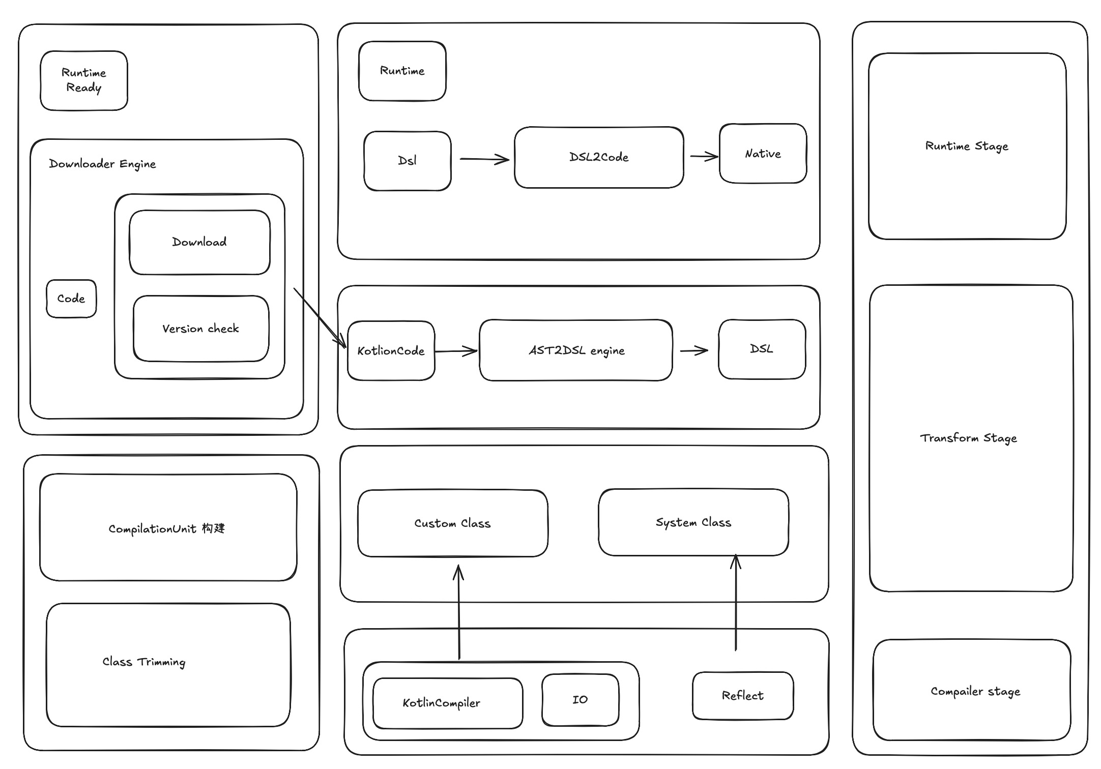 最下面的部分是编译依赖
- 中间是转换阶段
- 最上面是核心的runtime,runtime核心的是做一个类似于虚拟机的栈,保证所有的转换后的DSL映射后的对应数据,模拟成系统的栈结构。
三、困难
1. AST转换难点以及运行原理
AST意思是就是一个抽象的语法树,Kotlin的语法树与其他语言类似,但是还是存在差异,在Kotlin里,“org.jetbrains.kotlin.lexer.tokens”包含了所有的token。AST通过compiler解析语法树里的各个token值完成语法树的解析。
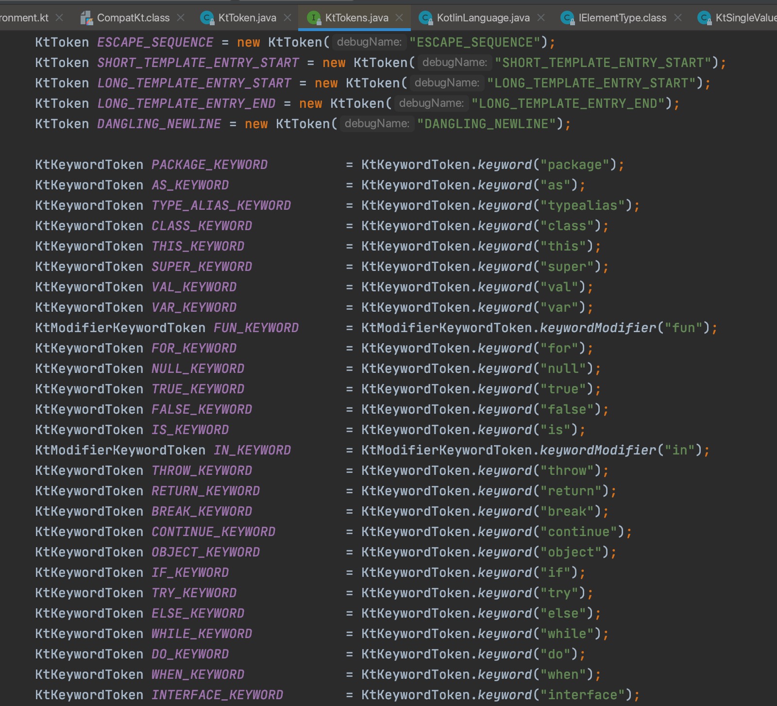
举个例子
object DemoFunctionExpress {
  /**     * result =10     * result2 =10     * index = 5     */
   fun test2(index: Int, item: String): Int {
    val a = 2
    val b = 2 + index
    return a * b
   }
}
如果不加以精简它是一个非常庞大的一个数据结构。
精简后。最后它的机构是类似于这种
KtFile (name: DemoFunctionExpress)
│
└── KtObjectDeclaration (name: DemoFunctionExpress)
    │
    └── KtNamedFunction (name: test2, parameters: [index: Int, item: String], returnType: Int)
        │
        ├── KtParameter (name: index, type: Int)
        ├── KtParameter (name: item, type: String)
        │
        ├── KtBlockExpression
        │   │
        │   ├── KtValVarKeyword (keyword: val)
        │   ├── KtNameIdentifier (name: a)
        │   ├── KtConstantExpression (value: 2)
        │   │
        │   ├── KtValVarKeyword (keyword: val)
        │   ├── KtNameIdentifier (name: b)
        │   ├── KtBinaryExpression (operator: +)
        │       ├── KtConstantExpression (value: 2)
        │       ├── KtNameReferenceExpression (name: index)
        │
        │   └── KtReturnExpression
        │       └── KtBinaryExpression (operator: *)
        │           ├── KtNameReferenceExpression (name: a)
        │           ├── KtNameReferenceExpression (name: b)
这个结构最外层就是一个progrem代表一个最小的程序单元,内层是嵌套一个KtObjectDeclaration,它表示一个函数的声明,再内部就是一个表达式和一些参数的声明,这个表达式最后其实就是一个将Kotlin的源码进行json化的一个转换。
生成上面的结构我们是依赖于KotlinCoreEnvirment的Visitor来进行解析,但是这个类的访问节点会遍历很多,所以我们我们需要对其进行精简,
举个例子,下面是一个二元运算的一个节点。
override fun visitBinaryExpression(
 expression: KtBinaryExpression, data: Void?): Map<String, Any?>? {
   println("Visiting binary expression: ${expression.text}")
     super.visitBinaryExpression(expression, data)
      return mapOf(
         "type" to "BinaryExpression",
          "name" to expression.name,
          "operator" to (expression.operationToken as KtSingleValueToken).value,
          "left" to visitNode(expression.left, data),
          "right" to visitNode(expression.right, data),
          "node" to expression,
           )
          }
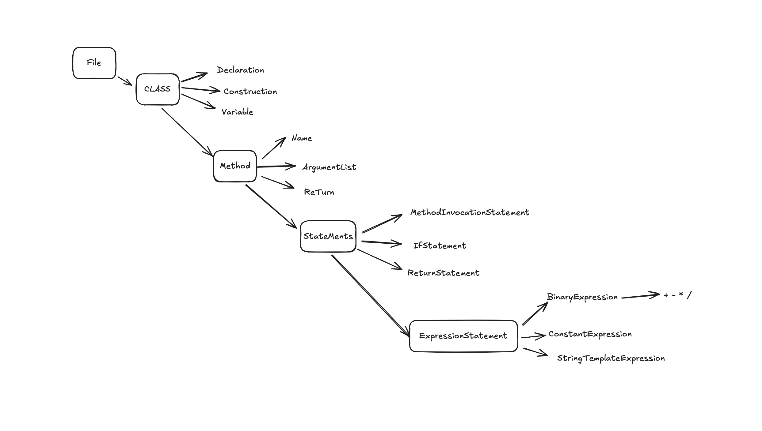
加载流程
当我们想要去加载上述的方法的时候的时候首先我们会将原文件加载到内存里,作为解释器的输入。
val test2 = runtime.invoke("test2", mutableListOf(5))
这一步我们是将AST转成DSL,然后我们会去遍历这个AST对应的所有的节点,然后精简成我们需要的DSL加载到内存里,这一步引擎会给他一个自定义的方法名并且与映射的方法产生一一对应的关系

它的执行流程简化来说可以是一个虚拟机的执行过程
- 在堆栈上查找名称为test2的方法
- 将参数分别压栈
- 遍历方法在是否在本单元内部->相邻类->系统类
- 找到后分别执行,退栈
- 返回结果
上述案例仅展示了 DSL 体系中的基础场景片段,实际应用需处理更复杂的 多维度逻辑嵌套,典型场景包括但不限于:
- 多层循环结构中的集合操作(如
O(n²)级联flatMap与状态化reduce的复合逻辑) - 异步回调链中的高阶条件分支
- 动态上下文依赖的 AST 节点生成(基于运行时元数据的子树构建)
受限于技术文档篇幅,本文未展开具体业务实现细节,但其核心机制具有一致性:
- AST 增强型描述协议:在标准抽象语法树构建阶段,注入 上下文感知处理器(Context-Aware Processor)
- 结构化数据组装:将转换后生成的 异构 Map 节点(Typed Map Node)按原始 AST 拓扑结构进行 递归归并(Recursive Merge),确保数据层级与源结构严格同构
- 工业级序列化方案:通过 预编译型 JSON 序列化组件实现 AST 中间表示到标准化 JSON 的高性能转换,可以提高加载速度,可以作为优化项目。
当我输入5
回看上面的方法
object DemoFunctionExpress {
  /**     * result =10     * result2 =10     * index = 5     */
   fun test2(index: Int, item: String): Int {
    val a = 2
    val b = 2 + index
    return a * b
   }
}
输出结果
val test2 = runtime.invoke("test2", mutableListOf(5,"a"))
System.out.println("动态化引擎输出结果:" + test2)
上述只是一个简单的数据处理,实际企业级的应用不可能是是这么简单的逻辑处理,我们可能还有自定义的加载类或者使用系统类,如何去保证这类能够完全的动态化呢?
apply方法
需要针对静态方法和非静态方法分别处理
fun apply(
            method: AstMethod,
            positionalArguments: List<Any?>,
            namedArguments: Map<String, Any?>?
        ): Any? {
            if (method.isStatic) {
               xxxx
            } else {
                xxxx
                throw IllegalStateException("error instance")
            }
            return null
        }
    }
静态方法可以直接使用方法名压栈处理
fun scopedInvoke(
       parameters: List<_ParameterImpl>?,
       positionalArguments: List<Any?>,
       namedArguments: Map<String, Any?>?,
       invoke: (List<Any?>, Map<String, Any?>?) -> Any?): Any? {
       val programStack = context.get<ProgramStack>(ProgramStack::class.java) ?: return null
       programStack.push(name = "parameters scope")
       parameters?.forEachIndexed { index, parameter ->
         if (parameter.isNamed) {
           programStack.putVariable(parameter.simpleName,namedArguments?.get(parameter.simpleName))} else { programStack.putVariable( parameter.simpleName, positionalArguments.getOrNull(index))}}
           val result = invoke(positionalArguments, namedArguments)
            programStack.pop()
            return result }
             }
           }
如果非静态方法,根据类的名称分别从相对路径自定义类或者系统类去加载对应的对象并且压栈
自定义类
对于自定义类,我们通过模拟类系统存储符号信息,在解析时将Kotlin的原始文件里的节点转换为可处理对象:属性声明转为Variable类型,方法声明转为不同类型的Function类型。
如果是相对路径重新生成对应的元信息node
if (newNode != null) {
        if (!dependencies.contains(newNode)) {
            dependencies.add(newNode)
            _visitNode(newEntity, dependencies, newNode)
        }
    } else {
        //反射

    }
在获取方法的时候通过加载刚刚自定义类的元数据完成
fun getClass(className: String): AstClass? {
    return context.run(
        name = "AstRuntime",
        body = {
            _program?.getClass(className)
        },
        overrides = mapOf(
            ProgramStack::class.java to { programStack },
            AstRuntime::class.java to { this }
        )
    ) as AstClass?
}
fun getClass(className: String, recursive: Boolean = true): AstClass? {
     //xxx
    dependencies.forEach {
        it.getClass(className, recursive = false)?.let { clazz -> return clazz }
    }
    return null
}
对于系统方法
最简单的就是反射传入类的方法和路径,精简反射的类的信息,通过getClass去构建一套基于系统的元数据结构。
经过层层拆解,最终还原一个精简版本的数据结构,用户下一步的处理
Scope上下文:
Scope 本质上承担着上下文环境的角色。当解释器对每个方法或表达式进行求值时,必须接收一个由外部传递的 Scope 参数作为执行基础。这种上下文对象具有链式传递特性:当前语句执行完成后,其可能修改过的 Scope 状态会成为下一条语句执行的输入参数。所以这里需要有一个跨线程的上下文,使用ThreadLocal维护,通过 Scope 的引用机制获取其存储位置,这种设计不仅支持数据属性的跨语句存取,还能实现方法定义的动态调用——包括方法内部嵌套调用其他已注册方法的场景。正是基于这种可传递、可扩展的上下文容器机制,系统才具备了处理用户自定义方法及其内部复杂逻辑的能力。
object AppContextManager {
   private val contextHolder = ThreadLocal.withInitial { AppContext(null, "ROOT", emptyMap(), emptyMap()) }
    // xxx
    val context: AppContext  get() = contextHolder.get()
    // 设置当前线程的 AppContext
    fun set(context: AppContext) {
        contextHolder.set(context)
    }
    fun get() :AppContext{
       return context
    }
    // 移除当前线程的 AppContext
    fun removeContext() {
        contextHolder.remove()
    }
}
context.run(
    name = " instance scope", body = {
        AstMethod.apply2(
            method,
            positionalArguments = mutableListOf(),
            namedArguments = mutableMapOf()
        )
    }, overrides = overrides
)
Card(
        elevation = CardDefaults.cardElevation(4.dp),
        modifier = Modifier.fillMaxWidth()
    ) {
        Column(modifier = Modifier.padding(16.dp)) {
            Text(
                text = title,
                style = MaterialTheme.typography.headlineSmall,
                color = MaterialTheme.colorScheme.primary
            )
            Spacer(modifier = Modifier.height(4.dp))
            Text(
                text = content,
                style = MaterialTheme.typography.bodyMedium,
                color = MaterialTheme.colorScheme.secondary
            )
        }
    }
它的结构简化下来就是如下样式,如果生成对应DSL更为庞大,这里就不展示了。
Compose Program
├── Composable Function: GreetingScreen
├── Composable Function: MessageCard
│   ├── Card 容器
│   │   ├── elevation 属性
│   │   └── Column 布局
│   │       ├── Text (标题)
│   │       │   ├── typography 样式
│   │       │   └── color 颜色
│   │       ├── Spacer
│   │       └── Text (内容)
简化流程:每一个组件都是对应的一个特定的语法树,语法树的解析,以来上文说的递归使用上面说的动态反射机制就能够还原这些View,
四、挑战
- 工作量巨大,需要保持耐心,笔者在业余时间进行探索,几乎已经全部时间进行投入。
- 项目较为复杂,核心链路虽然跑通了,但是一些复杂的语法还未支持,需要保持一定耐心去兼容,之所以开源出来也是希望依赖于社区同学一起投入进来。
- 因为牵扯到AST和DSL的转换和解析执行虚拟机的加载,对于排查问题有一定的门槛,边界异常逻辑处理需要后继者更为注意。
五、未来支撑的生态
虽然Aether的设计理念和效率上都有很大的技术创新和亮点,能够做到对于90%以上场景媲美原生,做到了真正的兼容性能与跨端和动态化的能力,并且整个链路最小单元已经跑通了,但是目前还是依赖于笔者一个人去开发,还缺乏一些脚手架,希望能够涵盖研发、调试、监控、测试、一体的建设。大图如下
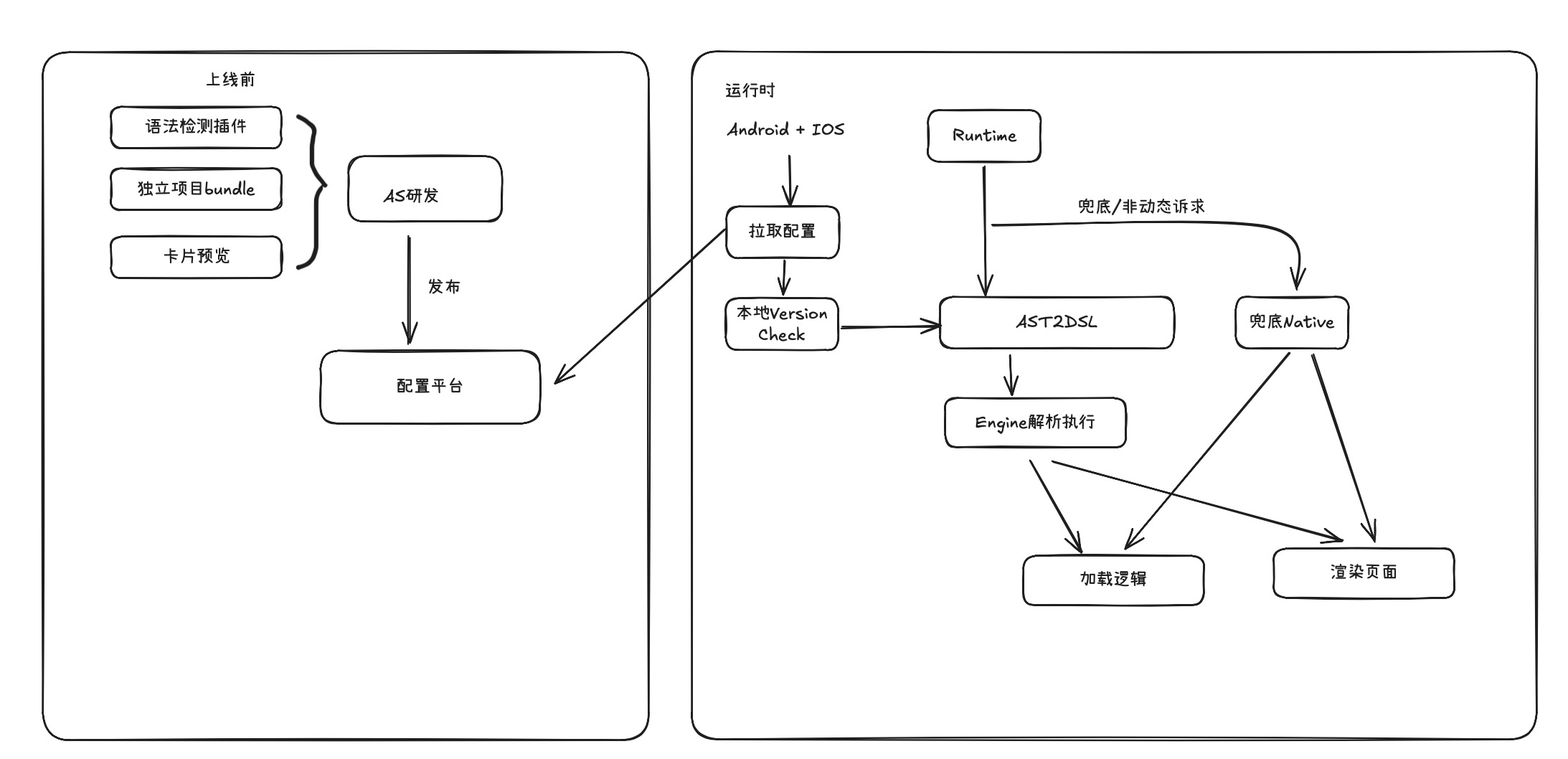
Aether 业内首次创新性基于AST + Runtime 构建KMP的动态化方案,实现逻辑页面动态下发,全流程覆盖开发至运维。提升发版效率与热修复能力,有效缓解KMP缺失的动态化,可大范围的推动Android KMP的生态发展,甚至可以革命掉现有Lynx和Weex的生态,但因为个人精力有限,还有很多工程化的能力需要建设,期待社区一起未来后续将强化复杂语法支持与生态建设,降低开发成本、优化体验并扩大业务覆盖;推进大前端融合,实现跨终端一致性体验。
 沪ICP备2025124802号-1